
Introduction
.
Much like the biological world is encoded by God through its cellular DNA—all living organisms are in this way specially encoded by Him—so too the nonbiological world is encoded by God through its electronic band structure. In this study we will discuss what these bands are and how they manifest in materials and why they are central to our understanding of how God’s good earth and universe per se operate.
It pleased our Creator to place us into a universe that consists of three sorts of “reallys.” One is what we like to call the “really normal,” another is the “really tiny,” and the other is the “really fast.” Really normal, really tiny, and really fast. We are like fish out of water in the really tiny and the really fast—the really normal is what we are best suited for. But there it is, and we must deal with it somehow, the really tiny and the really fast that is. This study of electronic band structure in materials is concerned with an aspect of the really tiny; let’s consider a couple of the “fish out of water things” therein first, and then slowly ease into our subject. Here’s a wet one: how does one accurately weigh a particle of dust if one might purely, i.e., without contamination, isolate the thing in the first place? We are not in the realm of the really tiny yet with this dust particle, it could even be argued that it is really normal this dust, but obviously not all that normal when it comes to measurement. Here’s another wet rascal: when two grains of sand collide, what is their recoil trajectory? How does one go about determining that trajectory? We are still pretty much in the realm of the really normal here, but again, not without significant challenges as concerns detection and measurement. Nowadays we have quite sophisticated instruments that help us out here, but even so, the whole procedure is far from normal. Now let’s get really tiny. Electrons and atoms—that’s really tiny. That “tiny world” is strange. Nothing “normal” works there as far as computations are concerned. One cannot even know with certainty where these really tiny things are at or how long they persist here or there—really messy… Well, it is a testament to the image of God within us humans and His abiding grace that we “done figured it out,” really, starting with the really normal stuff that took centuries to settle, and then gradually starting around the middle-ish of the nineteenth century we made significant strides in discovering (some of) the secrets of the “really tiny” and the “really fast.” Newtonian and Maxwellian mechanics got us off the snide, and then along came big progress in thermodynamics and ultimately quantum mechanics (QM) for dealing with the really tiny, and relativity for dealing with the really fast. Straightforwardly and simply, we are going to be talking about the QM electronic band structure of solids in this study, and will discover at the end of it all that it undergirds all of materials science and semiconductor physics by way of an elegant encoding that governs all the interactions of all the really normal stuff all around us—it is exceedingly good to say already that this is to Jehovah our Creator God’s glory this Elegance, really.
We are going to approach our subject in two ways, a “conventional” QM way, and our beloved feedback way; these two approaches dovetail into one another, but not just our bias forces us to say that the latter is easier, simpler, maybe more accurate, and certainly much more exhaustive and…more of a joy (at least to us) to implement, readily lending itself to computer modeling (it is a discrete idea after all). Okay, let’s really do it just now.
Definitions, Energy Bands and Gaps
First some clarifying definitions.
- A free electron is one that is not bound by some external force, thus free to move about and interact with its environs. For our purposes, a free electron has acquired enough energy to break free of the atomic lattice it connects with, hence it possesses much (kinetic) energy over against bound electrons “stuck” at lower energies.
- The fermi level (named after Enrico Fermi) is the highest energy level occupied by electrons at 0K (K for Kelvin, 0K is absolute zero temperature; we need a reference, at 0K all electrons are in their lowest energy state, then we can say things like, given no external stimuli, and ground states across the board, where would the theoretical location of such and such a band be—0K “floats all ships to the same baseline” if you will). The fermi level is sort of an imaginary energy dividing line, energetically above which (fermi level not inclusive) is what is called the conduction band (free electron band—higher energy because these electrons possess the “broken free of the lattice” energy) and below which (fermi level inclusive) is the valence band (lattice-bound electron band). The whole idea of electronic energy bands revolves around this fermi level metric. Notice that in the diagram metals essentially have no band gap, so in a sense it is meaningless to talk about energy bands in metals. In metals the valence band is partially filled with electrons while the conduction band is partially empty, thus there is room for movement from the former into the latter, and since the energy gap between these bands is largely zero, valence band electrons can easily “jump” into the conduction band in response to near nil stimulus and become free electrons. Since these electrons essentially have no energy restraints on them (no “lattice-leash”), true to their name, they are thus free to move about in the metal, which means almost immediate response, in the form of electric current (=KE), to external stimuli such as electric or heat energy, and that is why metals are such excellent conductors of electricity (and heat)—basically no band gap here. (The heat response is in the form of molecular vibrational energy that shadows the external source of the heat that ramped up free electron KE in the first place, which KE is transferred to other molecules in the metal setting the whole thing into a heat-generating vibrational state.) Nothing is ever gained for free in our Lord’s universe; an electron must be able to jump into the conduction band in order for interesting and practical things to happen, and some external energy must always be input into the system for that to happen—it is a hard and fast rule of God, nothing ever comes for free (unless He graciously gives it to us, like Salvation for example). It follows from the foregoing discussion of metals that insulators have no free electrons available, all electrons are bound/stuck to the lattice—the bandgap between the bottom of the conduction band and the top of the valence band is large here—much external energy must be introduced into this material to overcome that energy gap. The band gap between the conduction and valence bands in semiconductors is relatively small, but nonzero. With the introduction of chemical dopants into the intrinsic semiconductor material, this gap size can be manipulated and the fermi level can be shifted (the fermi level sits precisely in the middle between the valence and conduction bands in pure, intrinsic semiconductor material at 0K), to make a material behave more like a conductor or an insulator in response to external stimulus, and that manufactured fermi level shift is the main idea behind semiconducting electronic devices, because the position of the conduction band relative to the Fermi level determines whether an electronic device operates as a conductor, insulator, or semiconductor (please see again the diagram and notice the relative sizes of the band gaps).
- Conduction and valence band. In nonmetals, the valence band is the highest range of electron energies which electrons normally possess at 0K (the fermi level is the highest, it sits atop the valence band, which is fully occupied at that temperature). The conduction band in nonmetals is the lowest range of electron energies devoid of electrons until they are excited into this band from the valence band; once in this band they are free to move about and as such manifest electric current. As said already, “conduction and valence band” in reference to metals is somewhat meaningless, because conduction happens in one or more partially filled bands that alike have the properties of both the conduction and valence band—there is overlap, as shown in the diagram.
- A free electron is a conduction band electron if and only if it has acquired enough energy to “jump the gap” from the valence band into the conduction band.
Statement of the Problem, Applications
Here is what we are going to do and why. We are back to the really tiny problem. Assuming we have energetically free electrons at hand, and in keeping with the presumed way of attaining to electronic band structure causals, we want to know how a free electron in some nonmetal solid interacts with the myriad atoms all around it, some 10^23 atoms on average within striking distance (10^23 = the numeral 1 followed by 23 zeroes). This is a “really tiny problem” much more difficult than trying to determine the recoil trajectories of two interacting grains of sand as posited above. But why do we care about these bands, why do such a study? Practically, by God’s exceeding revelatory grace, such studies have led to the following.
- Band structure theory leads to a sound understanding of the electrical properties of materials (e.g., electric current is the flow of free electrons in a given direction).
- Design optimization of conductors, insulators, semiconductors, and superconducting prospects.
- Band structure theory explains how materials interact with light, thus broadening our capacity to build optoelectronics, photovoltaics, and lasers, and to find new applications thereof.
- Band theory is crucial to our understanding of magnetic phenomena in materials, with applications in data storage, MRI (magnetic resonance imaging), and more.
- Band structure determines how heat is conducted in materials, understanding that has led to design optimization in thermoelectric devices.
- The electronic structure of crystals and applications (e.g., piezoelectricity—the accumulation of charge in response to mechanical stress).
- Manipulation of band structure allows for the specific, optimal design of materials with the necessary properties for specific applications.
The above is just a short list; one could go on and on here. Suffice to say that band structure theory is the key that unlocks myriad practical applications for humankind, and we are much blessed by God through the revelation of this elegant and pervasive design concept of His, revelation by way of Him and His myriad servants down through the centuries.
The Conventional QM Approach
We must convey some modeling set up explanations first and fold in a little QM background for clarity. Quantum mechanics helps us deal with our “tiny-world problems.” There is no other “mechanics” that does so currently. QM is the starting point for tiny-world problems. The roadmap derived from those results may be traversed non-conventionally though, as with our feedback approach discussed later. Conventional QM computes via a second-order differential equation named after Erwin Schrodinger—the Schrodinger equation. Simply put, this equation has a time-dependent version (TDSE) and a time-independent version (TISE). The TDSE is the starting point from which the TISE is derived. We will be working with the TISE in what follows. We will break it down and try to make it conceptually manageable and pleasing.
It is an energy game that is played here. We spoke of an Action Principle (A) in another study. A=kinetic energy KE minus potential energy PE (A=KE-PE). Here we have a different sort of “action,” though it is not properly an action in the strict sense. Here, instead of subtracting PE from KE, we add. Here, we are interested in total energy, called the Hamiltonian (H, named after (W.R. Hamilton). The TISE is rooted in H. As said, H is not an action in the strict sense, it is what is called an “operator.” And operators, guess what, operate on things; they are very “order of operations” sensitive. For example, multiplication is an operator—the operation is the multiplication of things (1x2x3x4=24—an arbitrary multiplication operation; multiplication is not order sensitive though—the answer is the same no matter the order of operation). H operates by way of differentiation and addition. More specifically, proxied by the TISE, it takes the second derivative with respect to (wrt) space—by definition a curvature—of a wave-like thing, and adds to that some other thing times that same wave-like thing. So that is how H operates—you give it those two things, and it operates exactly as said. And what happens is that this operation is tantamount to a kinetic energy KE (the first operation, the second derivative wrt space) and a potential energy PE (the second operation, the addition). And KE+PE =total energy E. Clearly, H encodes interactions via energy considerations. That is axiomatic and fundamental to band theory. Here is what we mean in the context of our tiny-world problem of free electrons interacting with the myriad atoms in their environs. When such an electron encounters an atom its energy (KE+PE) changes, and those changes betray, i.e., describe, the interaction. Since H, the energy operator, is precisely that very energy, one can predict how interactions will occur given various boundary and starting conditions fed into H. We will be making such predictions shortly to make these words more explicit.
In the context of our free electron-atom interaction problem, to make the problem as simple as possible, we are going to assume that we are working with crystalline material, i.e., a regular array of atoms (please disregard the controls on the sides of the checkerboard lattice for now, also the verbiage at the top comes into play later—they are for use with our feedback model). In the diagram we show a checkerboard-like crystalline atomic lattice. The dark cells represent arbitrary atoms of the same kind surrounded by their peculiar electron cloud (cloud electrons are not necessarily free electrons—they are bound electronically to the atoms of the lattice comprising the material at hand); so, the dark cells represent both the nucleus of the atom and the peculiar electron cloud surrounding the nucleus. The light spaces seen in between the atoms are force-free spaces, i.e., no potentials there (force is a function of potential by definition). And of course we expect two things to happen when an electron in this lattice receives enough external energy to break free of it and become a free electron, it will strike another atom, and it will traverse spaces between atoms. Our modeling of this tiny-world action will necessarily involve both cases; it will be modeled first by way of a conventional QM approach as said, and then via our feedback approach. The crux of this study comes together in that modeling, and that is what we have been providing background for all along. Since the space between the atoms is assumed to be potential free, the Hamiltonian H will not have a PE term in the spaces, only a KE term. But if the free electron strikes an atom, an interesting assumption will be made, that goes like this. We are going to lean on a slick little function that Paul Dirac conceived of, called a (Dirac) delta function. That function has this mathematical property (entirely a clever and handy and mathematically sound abstraction—nothing real here): whenever it “sees” a zero, its height, i.e., magnitude, at that zero spikes, whilst its width narrows to maintain a constant area of precisely 1. So, if we map the electron-atom interaction energy to a distance of separation delta function, then when the electron strikes the atom, we will assume that the energy of interaction has spiked to 1 (or whatever value we assign to the strength of the delta function) because upon impact the distance of separation is precisely zero.
To sum up our conventional QM modeling approach set up, we have the following.
- The material in which we investigate free electron-atom interactions, ultimately to see free electron energy bands and gaps that manifest, is crystalline, consisting of a regular array of atoms of the same kind. We will use this periodicity/regularity to our advantage in the model.
- QM will (must) guide the analysis; the TISE, rooted in H—total energy—will allow us to predict how the free electron energies change in the potential-free spaces between the atoms—a KE dominant energy, i.e., motion related, is expected, and a Dirac delta function will guide how the free electron energies change upon striking an atom—a spike in their potential energy. The tools we are using are QM energy tools because we are interested in energy bands and gaps manifestation in the real-world scenario of free electron interactions with an atomic lattice—really tiny-world stuff that calls for a different approach to computing than the “really normal” tools have to offer in the way of computing anything of integrity in this strange tiny-world that seamlessly functions behind the scenes out of sight in lockstep with the really normal world all around us. It is a breathtakingly amazing synchronicity and God our Creator be praised for it amen and amen.
Next, we will do and show what has been written in words. It is not necessary for the reader to follow all the QM related mathematics that we will show, please feel free to skip all that without loss of generalities and jump to the concluding comments section.
The Conventional QM Band Structure Model
Since we know what happens when a free electron encounters an atom—a spike in its potential—our starting point is discovering what happens to it in the spaces between the atoms. It turns out that its motion is like a pinball bouncing back and forth from a couple of obstacles—back and forth, back and forth, cyclically, captured by a sine and a cosine term added together, A Sin[kx] +B Cos[kx] (Fig. 4 just past middle). Of course it is trapped, somewhat like being in a maze, hence the almost to be expected cyclic nature of its motion in the spaces. Though it is a crucial part of the solution, we are going to skip a detailed discussion of the discontinuity effects presented by the delta function, and at the edges. We have worked them out and will simply show them to the reader (Figs. 5, 6, 7, 8). Looking at figure 8 we see that we have some equations to work with now to move us forward, but we have a bunch of unknown coefficients that need to be determined first (Fig. 9). And some final “house cleaning” brings us closer to our solution (Fig.10). And finally, the conventional QM Band Structure model solution in figure 11–in figure 11 the horizontal axis is mapped to energy through k (Figs. 4, 11).
The Feedback QM Band Structure Model
QM is still the starting point—we use precisely the same equation for the free electron in the spaces (A Sin[kx]+B Cos[kx]), and upon striking an atom a delta function potential similarly spikes, all that is the same. The difference comes by way of implementation, which sees things from the free electron’s perspective, i.e., unhindered by differential calculus stumbling blocks. So here we try to simulate an actual free electron hitting the lattice, and whatever happens, does so under feedback. What we would like to say in this section is best said by way of demonstration in a short video. In the video we incorrectly say that with a lattice size of 40×40 there are 800 atoms, the correct number is 400, i.e., 1600 total cells on the lattice, but taking into account the spaces, that number divides down by a factor of 4. In the final plot the coloration goes like this, since the original lattice was a checkerboard that goes: space, atom, space, atom… across each row and down each column, the coloration follows suit, there will always be an atomic spike next to a sine[kx]+cosine[kx] trig response in a potential free space, across each row and down each column, and the spikes will consistently show up as a sort of reddish-brown color, and the potential-free spaces will be of varying colors depending on their Pythagorean location in the lattice (the x in sine[kx]+cosine[kx] is a Pythagorean distance, where {0,0} is at the center of the lattice). The final pattern shows some of these potential free spaces as a sort of grayish ring–that’s a band (conventional QM has the k in sine[kx]+cosine[kx] mapping to energy), and interspersed around and in these rings are reddish-brown spikes and other colors–tan, yellow, golden, light blue, etc. representing spaces, altogether forming bands in between bands–bunches of concentric rings(Fig. 12).
Concluding Comments
Starting with a tiny-world problem of electron interactions with an atomic lattice, we have tried to show in this study how electronic band structure in materials manifests. Quantum mechanics guided the study throughout—those ideas and equations were fundamental. QM is the only way possible to deal with tiny-world problems such as these sorts of interactions, at least as of today. But we also wanted to show the action on the lattice, and that was the feedback. So, QM for its part is indispensable as per the guiding equations, but the feedback is no less indispensable for taking that next step and doing things in situ real-time. The two work together well to do “real world” modeling.
Finally, let’s take a step back and focus on our Creator. Materials are encoded by God in the language of energy. And where does energy come from but from God, let alone its clever utilization, amen. Electronic band energy identifies a material, and it sets bounds on how, and with what other materials, a given material may interact. They are like fingerprints these energy bands as far as identification goes, and they are like precisely hewn keys as far as unlocking interactions with other materials goes. It is the work of a powerful, surpassing genius, none other than Jehovah our God.
Praised be your elegant Name great Jehovah God, whom we love and adore. Amen.
Illustrations and Tables
Figure 1. To unlock, to shake hands, materials’ bands and gaps must be precise.

Figure 2. A Regular Array of Atoms—A Crystalline Lattice.

Figure 3. Fermi Level.

Figure 4. Psi and E (energy E is in terms of k) in Spaces (potential V=0 there).
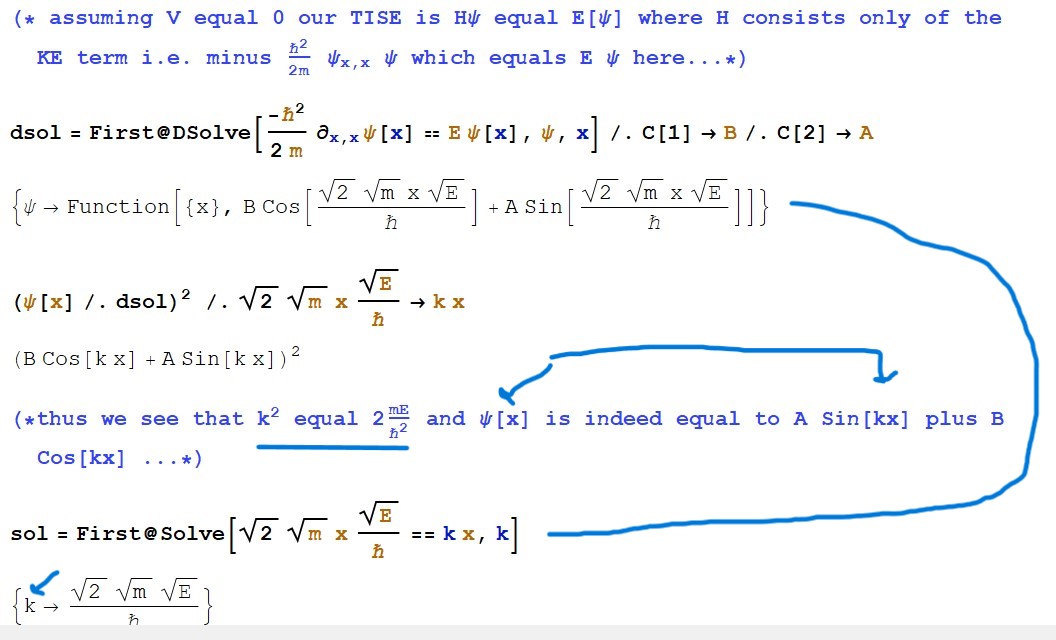
Figure 5. Preserving Continuity across the Delta Function.
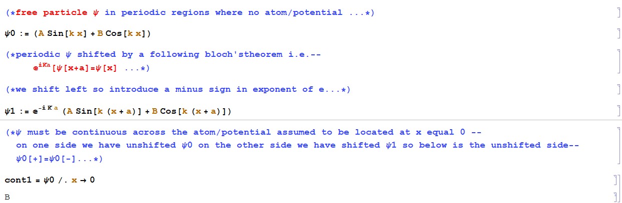
Figure 6. Preserving Continuity across the Delta Function cont’d.

Figure 7. The Discontinuity.
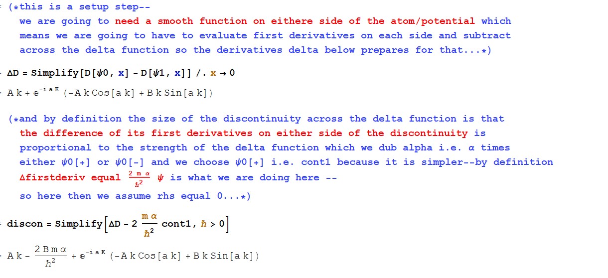
Figure 8. Preserving Continuity Recap.

Figure 9. The Coefficients—below references Figure 8.

Figure 10. Last Steps (not shown—K=2npi/Na, N ~10^23, a =atom separation).

Figure 11. Crystalline Free Electron Band Structure (=allowed energies).
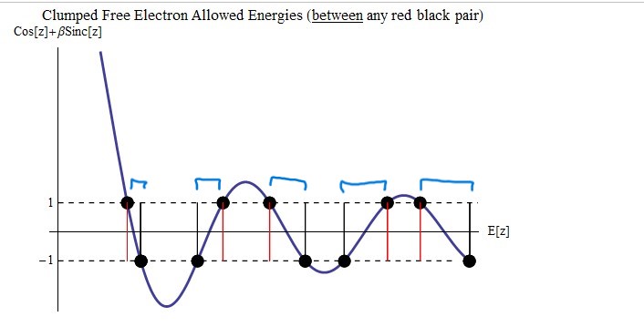
Figure 12. The Feedback Model.
Works Cited and References
“A Letter of Invitation (not cited, always a standing invitation).”
Jesus, Amen.
< https://development.jesusamen.org/a-letter-of-invitation-2/ >
“Creation Action.”
Jesus, Amen.
< https://development.jesusamen.org/creation-action/ >
“Dirac Delta Function.”
Wikipedia.
< Dirac delta function – Wikipedia >
“DNA.”
Wikipedia.
< DNA – Wikipedia >
Griffiths, D.J.
Introduction to Quantum Mechanics.
Reed College Oregon, 2018.
“Valence and Conduction Bands.”
Wikipedia.
< Valence and conduction bands – Wikipedia >
“Electronic Band Structure.”
Wikipedia.
< Electronic band structure – Wikipedia >
“Fermi Level.”
Wikipedia.
< https://en.wikipedia.org/wiki/Fermi_level >
“Free Particle.”
Wikipedia.
“Hubbard Model.”
Wikipedia.
“Schrodinger Equation.”
Wikipedia.
< Schrödinger equation – Wikipedia >
Wolfram Research Inc.
Mathematica.