Introduction
Here we find another very elegant example of optimization in the created order (nature henceforth). Nature, per the design of the Creator God Jehovah, seeks to minimize its action, or better, it seeks to find stability—let’s call it A for action. Simply put, A is how a system changes over time, and nature seeks to minimize this change, this A. For example, an object (the “system”) may be at rest initially, then undergo some gyrations, and finally come to rest again after some amount of time has elapsed—it is those gyrations that are minimized like “clockwork,” automatically, always. A golf ball is at rest on the tee. It takes off in flight after the golfer strikes it with a club, it follows a parabolic trajectory while in flight, then comes back down to earth again and bounces for a while and rolls somewhat, and finally comes to rest. A involves the time between the ball at rest on the tee and hitting the earth somewhere downrange in this example; in particular, the time in flight is minimized, nature “computes” the least time trajectory by way of minimizing the action. We are only concerned with that least time trajectory in this study and will ignore the rest (the bouncing and settling and whatnot, which is outside the domain of A). Stability by way of minimizing A is intimately associated with energy balance. Energy may be in the form of kinetic energy KE, which bespeaks motion, which bespeaks instability, for as long as there is motion there is change and hence there can be no stability, or it may be in the form of potential energy PE, which bespeaks potential change, not actual change, which bespeaks stability until that potential is realized. In the mid eighteenth century two mathematician/physicists, Leonard Euler and Joseph Louis Lagrange, derived an equation per God’s grace subsequently named in their honor called the Euler-Lagrange equation (ELE) that reasonably captures how A is minimized in nature. The ELE is a gem and goes something like the following.
ELE, Lagrangian
A is analyzed by way of an energy operation called the Lagrangian (referred to as “L”). L operates at all points along a given object’s path of motion (along some trajectory). We will show L to be a summation of object energy along said trajectory; actually, it is a sum of energy differences at all points along a given object’s trajectory, as will be shown. One of the main motivating questions that prompted study in this field, already in Isaac Newton’s day[1], was this: How is it that nature always seems to prefer certain trajectory shapes? For example, how is it that launching a projectile at a certain angle, like our golf ball above, follows a parabolic path from the launch point until it finally lands somewhere downrange? Why not some other trajectory shape, say sawtooth-like, i.e., straight up at an angle, then straight down at an angle, sort of a “kinked” trajectory? Newtonian mechanics explains how no problem, but that only works for near-earth trajectories, because the gravitational force on objects is not constant, it varies inversely with distance from the center of the earth, and thus the acceleration of the object varies as well, being greatest the closer it is to the surface of the earth[2]. As practical a tool as it certainly is, we need a more precise analytical tool than Newtonian mechanics in our action-quest, and the ELE is that tool; it is extensively utilized in (classical) analytical mechanics, but finds applications in quantum mechanics as well, e.g., determining the bound energy eigenstate ground state for a delta function potential wave function.
The ELE is derived from a consideration of energy “trade off,” as captured by the Lagrangian L. L is simply kinetic energy KE minus potential energy PE (L = KE-PE), at all points along a given trajectory, where each L for every point along the trajectory is determined at a given instant in time, an instant we call “dt.” Positive Ls mean KE dominates, negative Ls means PE dominates. So, all we are going to do ultimately is add up all those differences at those points. And we are going to force each point along some “test” trajectory to be only a very tiny distance removed from its neighbors. With that in mind, please take another look at the red font L if you will and ask, how would I minimize L along some trajectory? It seems reasonable that if one could somehow force an object’s motion to linger in regions where the PE is high and zip along regions where the KE is high, that should minimize L for us (and in turn A, because A is comprised of a sum of Ls, one for each time slice dt during the motion). That answer in fact gets at the heart of what we are going to show, more mathematically, below. (The reader may skip the math grunge and jump straight to the examples section or the theological section without loss of continuity for our purposes in this study.)
In the diagram we consider three points a, b, and c out of myriad points along a line, where a and c are not variable, i.e., they are fixed/locked in place, and b is variable (Fig. 1). Here is what we are doing: We impose a local change on our test trajectory (the solid, straight line in the diagram), so we pull up at point b to create a “corner” as shown, and this imposes a change in L at point b because b is now up higher, its L (KE-PE) value has changed (change plays the role of the “villain” in minimizing A). And we want to understand how the neighborhood around the raised b both looks and behaves.
For starters, we see two dashed line slopes oriented differently on either side of the raised point b (Fig. 1). It tells us that all the points that comprise those slopes have different L values (they are on a slope after all—for every tiny step in the horizontal direction, left or right, there is a change in L, whereas before we pulled up at b, L was not changing along the solid line, it was zero everywhere: no KE, no PE). But notice, at the raised point b we have a minimal L and stability (these go together “like a hand in a glove”). But exactly why ?
(1) At that point L is minimal because it is relatively more negative than at the other points on either slope because it is purely PE there (the figure shows the absolute value of L, hence all positive; the relative magnitudes of L are changing along the slopes at a constant rate, and we are most negative at the tip of the red arrow, i.e., no KE related motion there).
(2) Stability follows because L is no longer changing there.
That is the genius behind the ELE, in this manner, with more detail forthcoming, it manages to eliminate all the KE (the change villain) along the trajectory, with integrity. But how? If we could merge points a and c with point b, then pulling on b would effectively lift the whole test trajectory with minimal slopes depending on how closely we could bring, in the end, all the points together. In fact, if the points were “infinitesimally” close together, we could preserve continuity from one slope, around the corner, to the other slope. We would then, in keeping with the L summation definition of A, add the L values of the two slopes and the stable point b, precisely at the points-merged point b. Again notice that the dashed line slopes are oriented differently (left is positive, right is negative, Fig. 1), hence their sum is effectively a difference, a difference in slopes. Now the important thing to be noted is that bringing all the points together by some small distance happens in time; yes, the points are brought together in space, but of course during some time slice dt. Therefore, if our merging produces a difference of slopes around the corner, it does so as a difference with respect to time, and differences per time are referred to as rates (of change). So, by infinitesimally merging our points, we realize an action A that is the sum of only two Ls effectively, an L for the stable point at the raised point b, and an L that is the rate of change of the two slopes’ L. So what is the next logical step? We want to subtract off the rate of change of the two slopes’ L from that of the stable point at the raised point b to effect stability despite local change. And then we repeat this process not just at some arbitrary point b, but at all infinitesimally separated points along the solid line test trajectory. That, in words, is what the ELE is doing. Mathematically, in the language of our “point merging infinitesimals,” it looks like this:
dA/dxb=0=dL/dxb-d/dt dL/dslopeb,
where (dA/dxb)=0 on the left is a mathematical statement of minimizing A, i.e., forcing stability by way of the part to the right of the 0, where the red font term corresponds to the stable raised point b—which represents PE, which we said earlier we want to keep and exploit—and the rest subtracted from the red font part is the time derivative of the change in the slopes across the corner, i.e., the rate of change of the slopes around the corner (=the KE villain), which we said we want to eliminate from the L that comprises A, so we subtract that part from the stable red font PE point as shown. The part to the right of the red font term that is being subtracted comes together as a second derivative, and second derivatives are decidedly a statement of curvature, so one could say that we are subtracting any motion-inducing curvature off the stable raised point b, and that in the end is the goal to be repeated all along the solid line test trajectory. This repetition at all points along the solid line test trajectory comes about by integration: considerations of minimizing A such that dA/dx=0, where A is given by the integral[ L dt] |12. In general, “Integral” here means a summation from 1 to 2 per some pertinent differential dt or dx or whatever depending on the problem at hand, where in our case that differential is dt, and 1 and 2 represent two distinct times, a beginning time (e.g., golf ball on the tee) and an ending time (golf ball hitting the earth downrange), the difference of which comprises the amount of time necessary to traverse the given trajectory. So bottom line, “integral” represents a summation with respect to differential time slices dt in our problem; we are adding up all the stable “PE points” and subtracting off all the unstable neighborhood “KE curvature” at every conceivable instant in time from t=1=time at the beginning of the trajectory to t=2=time at the end of the test trajectory.
Finally, we have been talking about stable trajectories and minimization of the A that produces this, it is referred to as “the principle of least action,” and the stable curves themselves are referred to as “stationary” curves. This sort of minimization is more challenging than simply finding a point minimum, because here one must “minimize” an entire curve to minimize A. It should be noted that the principle of least action is applicable across the sciences, classical and quantum, and as far as we know it is useful for problem solving across the board as it were. Its only drawback is its differential nature—we mean the human expression of the principle, not the principle itself, and hold that feedback via discrete computation is a better expression of it. Rule-based feedback provides both the means for computation, and the means for it to persist in nature—nothing happens for very long without it at work. (Wherever our Creator has His action code at work, He has His feedback code at its side and vice versa.)
Examples
Brachistochrone
A brachistochrone, literally “shortest time,” is an experimental gadget consisting of a bunch of (frictionless) tracks of different trajectory, one places balls at the top of each track, and then when hitting the “go button” all the balls are released and follow their track downward to the finish line as it were. The solution by way of the ELE and the calculus of variations of the “fastest track” (Fig. 3) is a shape like that traced out by a point on a rotating wheel moving linearly—a cycloid. In other words, it is the track that sort of slopes flat and a little up at first, but then slopes down precipitously (Fig. 3a), which means that A is minimized here because the ball spends more time on the flat portion with increased potential energy PE which tends to decrease A, and then it spends less time on the down sloping part where there is great kinetic energy KE (KE tends to increase A), and when one sums KE minus PE across the whole track A is minimized because one gets a lot of PE up front and the KE ‘ kicks in’ only relatively briefly. So the cycloid is the least time track. Nature seeks out these trajectories by default, case in point is light—light always finds the least time path, which is not necessarily the least distance (Fermat’s Principle).
Power Profile in an RC Circuit
This example is intended to show that the least action principle is not limited to literal kinematic type problems—nature operates the same in other settings. Given an electrical circuit comprised of a resistor R, a capacitor C, and a power source (an RC circuit), then the electrical power Lagrangian L is:
(q’)^2 R minus q/c,
where q is charge, and q’ is a first derivative of charge with respect to time (dq/dt)= current, and where the resistor R sinks the i^2 R =(q’)^2 R power (=KE for our purposes), and the capacitor provides the (q/C) PE (Fig. 4). As shown, the power drain on the source ramps up immediately as the capacitor charges through the load R, then it drops precipitously once the cap is fully charged, at which point (the peak—first derivative =0) the current reverses and flows in the other direction, sourced now by the cap, therefore the positive going portion of the curve is of interest as far as power drain on the source goes; we arbitrarily assign R= 1 kilo-Ohm, and C= 1 micro-Farad, thus the RC time constant of this circuit is one millisecond (RC is tantamount to time, it is the time required for the current to rise or fall through about 67% of its maximum amplitude, which happens exponentially). Nature computes these responses automatically, e.g., the human nervous system/brain activity, positive feedback oscillators. A natural analog of electrical resistance is mechanical friction, and that of electrical capacitance (capacity to store charge) is the (mechanical) compliance of a spring (the inverse of its stiffness, i.e., extent of non-deformation in response to applied force), and nature is fraught with these sorts of RC circuits and ever toils to minimize their response action—it is an optimization coded into nature, highly efficient, exceedingly elegant.
.
Light Ray in Medium of Variable Index of Refraction
By way of introduction to the subject, particularly the terminology, the index of refraction “n” is defined as the ratio of the speed of light in vacuum “c” to the speed of light in a given medium “v” (n=c/v; it is a relative measure of how fast light can transit a given medium, large index values n translate to lower speeds of light v [relative to the vacuum speed c]; this does not violate the special theory of relativity because c is ever fixed in vacuum). The index of refraction n is always greater than or equal to 1.0 (there is no upper limit), where 1.0 is the index of refraction of vacuum; the speed of light in a medium (v) is always less than its speed in vacuum (c).
This refraction example has no PE considerations to work with because a photon of light is massless, so we consider only the KE in L. We still want a shape that reduces this KE, but we have no PE offset this time.
As said above the relationship between the index of refraction and the speed of light is given by the formula:
n = c/v,
where n is the index of refraction, c is the speed of light in vacuum, and v is the speed of light in some medium. But in differential form v= differential distance/differential time= ds/dt, which therefore equals c/n, and we want to make stationary the Integral [dt] = 1/c [Integral [n ds], and the motivation for making the Integral [dt] stationary, i.e., an ELE operation, follows from Fermat’s principle:
the path taken by a light ray between two points is that which takes the least time.
Thus our functional (by definition, the stuff inside the integral brackets) is actually going to be r^-2 ds, not n ds, since n is inversely proportional to the square of the radius as stated in the problem objective above, so we replace n by r^-2 in the functional, and the radius r is some distance into the medium (some distance along any of the black arrows, which represent light rays). And working in polar coordinates, we know that differential distance ds= Sqrt [dr^2+(r theta’)^2]= Sqrt [ 1+r^2 theta’^2] dr upon division by dr^2 inside the square root, where theta’ is a first derivative of angle theta with respect to r because our differential has become dr owing to the division step. Our ELE solution and attendant plot follows from the foregoing set up.
The Creator’s Action Finger
The principle of least action is applicable to far more than test trajectories, it applies to any function, i.e., any “machine” that produces a specific output given a specific input (stimuli | response), and it is at work constantly all over nature (negative feedback forces it to persist per context-specific rules). The principle of least action is the reason is why things “look” the way they do—our world’s shapes are not happenstance—they are being forced to look like they do per this principle, and they always end up being the same shape in their contexts of action (for more on our Creator’s shapes, “Jehovah’s Conic Section Templates,” ”God’s Amazing Water”). Thus it pleased the Creator to extend to humankind the beauty we see around us by way of this elegant code He wrote into the dynamics of nature. How does the golf ball “know” it should follow a parabolic path? Do it and the earth “talk?” Newton gives us the equations, but that is not the answer we seek, because those equations only describe the trajectory, no more. ( Newton’s equations are informed by the principle of least action, action is primary, Newton’s equations follow from that is meant). The golf ball is ”stupid” if you will, so is the earth, yet without minimizing the action, who knows what sort of trajectories they might follow. There is an action code at work, and that code did not originate in these objects—they are inanimate after all, and moreover could care less about “survival,” they have no need whatsoever to survive and cook up some sort of optimization like minimizing the action for their ultimate good—the notion is absurd and must be dismissed. Let us recall that the principle of least action verifiably holds across the board in the sciences, classical and quantum—as far as we know everything is governed by it. How can that be, where did it come from? Either from the “stuff” of this so-called everything, or outside of this everything, those are the only two possibilities. But please note that this is a code as we have tried to show all throughout, the action principle is not “stuff.” There must be an intelligent, and not least very powerful agent (per the mass-energy the code operates on) behind it, that is the only thing that makes sense. Or maybe someone will say, hey, the principle does not hold for everything—well, that remains to be seen. Jehovah God by way of specifically Jesus Christ is that Agent no doubt about it on our end.
Praised be your elegant Name great Creator God Jehovah, whom we love and adore. Amen.
Illustrations and Tables
Figure 1. Test Curve Corner
Absolute [L] in the vertical direction, L is zero along the solid line, motion along dashed lines, no motion at tip of red arrow.
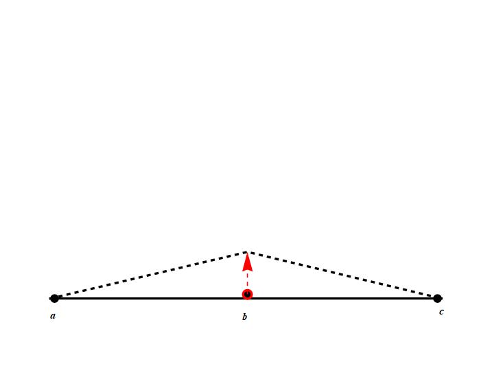
Figure 2. A Brachistochrone.
(Greek: “ shortest time”).

Figure 3. ELE Brachistochrone Solution.
(c is not related to light, it is a parameter that affects the size of the cycloid, arbitrarily set to 1/3 in the plot, x is the dependent variable, y the independent variable):

Figure 3a. The cycloid shape.
(huge lingering PE top left, huge precipitous KE right middle and down, this shape best minimizes brachistochrone transit time—nature computes these curves automatically on the fly in any conceivable setting).
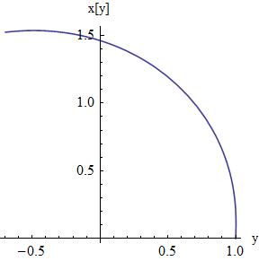
Figure 4. RC Circuit Power Profile.
ELE solution being plotted: q[t]= (3t+4RCt-t^2)/4RC, t is time, RC is the time constant. In the ELE computation q was the dependent variable, t the independent variable. Just like the golf ball mentioned above defaults to a parabolic trajectory in consideration of minimizing A, here the charge on the plates of the cap will always respond as shown given the parameters utilized in the circuit. In consideration of the curve shown, if this were the path of a golf ball in flight (it is not of course), then notice how the PE ramps up at the outset and lingers for a little over three seconds, then the KE takes over and by the fourth second, just one second later, the slope of that KE is approaching the vertical, and by the fifth second it is nearly vertical, which means almost no KE from that time forward, which gives us the best minimal A possible. Something similar is happening in the capacitor, its plates are being populated with charge at the outset which ramps up the PE, then when the cap is fully charged PE gives way to KE as the charge leaves the cap in the form of current through the load in the other direction. Nature demands it to be (to look) this way and no other way.
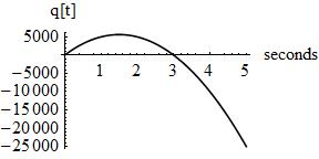
Figure 5. Variable Refraction Index n, Diagram

Figure 5a. Variable Refraction Index, ELE Solution.

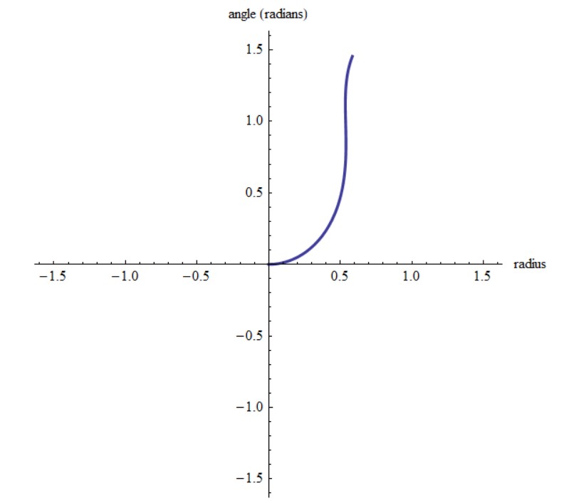
Figure 5b. Variable Refraction Index, Polar Plot.
The change in angle with changes in radius r is our KE, and it is incredibly steep, it is a fast transit through the medium by the light ray, precisely the least time transit. Our ELE functional was based on a time integral, time was the action of interest, and so our shape in this instance is a least time shape. Given a medium whose n value changes inversely with radius^2, a light ray will bend away from its direction of propagation (the black arrows) almost immediately going by the very short distance that the curve below is flat—it starts to turn up at 0.2 units and it is almost vertical at 0.5 units. The light is “hunting” for a least time path by way of bending and contorting as it transits the medium, bending and contorting away from the direction of propagation, laterally, vertically, you name it. How does it know it should do that? But of course, the Creator Jehovah must have His light transit optimally else His universe would implode.
Works Cited and References
“A Letter of Invitation.” (Not cited,ever a standing invitation in all that we do.)
Jesus, Amen.
< https://development.jesusamen.org/a-letter-of-invitation-2/ >
Boas, Mary, L.
Mathematical Methods in the Physical Sciences.
New York, 1983, John Wiley and Sons.
“God’s Amazing Water.”
Jesus, Amen.
< https://development.jesusamen.org/gods-amazing-water-transcript/ >
“Jehovah’s Conic Section Templates.”
Jesus, Amen.
< https://development.jesusamen.org/jehovahs-conic-section-templates/ >
“Creation Optimization.”
Jesus, Amen.
< https://development.jesusamen.org/creation-optimization/ >
Wolfram Research Inc.
Mathematica.
[1] Born December 1642, Newton flourished during the scientific revolution of the seventeenth century. He was maybe the first to utilize the Calculus of Variations (COV) of which this study speaks, per a solved problem published in 1687 in his Principia Mathematica, which he left unexplained as to the details of the solution, thus the disconnect between himself and the COV because no one at the time understood how he solved the problem.
[2] Classically, Fgravity = GmM/r^2, where m is the (constant) mass of the object, and M is the (constant) mass of the earth, G is the (Newton’s) gravitational constant, and r is the (variable) distance of the object from the center of the earth. One variable, the rest of the parameters are constants. As can be seen, gravitational force varies inversely with the square of the distance r from the center of the earth. At the surface of the earth the acceleration due to gravity ag, simply dubbed “g,” is assumed to be roughly 9.81 meter/second^2, where the exact acceleration depends on one’s elevation (and some materials factors). Force per se follows Newton’s second law: Force = mass of object times acceleration (F = ma, or, a = F/m as per acceleration), so we can rearrange the Fgravity equation above to get a feel for the gravitational acceleration on the earth in terms of the Fgravity equation parameters, and we do this by dividing out the mass m of the object, and we get: Fgravity /m = ag = g = GM/r^2 directed toward the center of the earth. We see that the acceleration due to gravity is object mass independent, it depends only on the constant mass of the earth M and the object’s variable distance r from the center of the earth (and the gravitational constant G coming along for the ride). Since the acceleration is object mass independent, then notwithstanding air resistance, two objects of different mass, say a feather and a brick, dropped at the same time from the same height, will accelerate toward the center of the earth with the same acceleration profile and hit the earth at the same time.