
Introduction
The ol’ yield curve may bend, its signals may sway,
still this not-so-little metric flat lights up the way.
Like shoe-leather maps, even stories that teach,
that rollin’ ol’ yield curve shows what’s out yonder in reach.
Best give it its due wise friend—this rascal ain’t never lied,
just wait out the noise, and let this here signal decide.
And so, with our eyes on the yield curve, this study is offered to the Christian investor as a guide through the tangled signals of the financial markets, much like a circuit tuned to clarity rather than distortion. May it bring blessing and peace of mind through clarity to all who read—Christian and non-Christian alike—and may our Lord and Savior Jesus Christ be glorified by it, for it rests upon His clear, righteous principles.
Alright then Beloved, here we go. Just as Scripture teaches us the rhythms of sowing and reaping in God’s Economy, i.e., in His Created Order (Job 4:8; Psalms 126:5; Proverbs 11:18; Ecclesiastes 3:1–2, 11:6; Hosea 10:12; Galatians 6:7, 9; 2 Corinthians 9:6, et al.), so too our economies move in a rhythm, in cycles. This should not surprise us, after all, economies are constrained to follow—at best—the Divine Rhythm. Said differently, whether we speak in poetry, policy, or practical power- pathways (circuits | physics), the truth is the same: economies cannot escape the rhythm set by their Creator—they can only follow it, at best. The challenge is not to eliminate these cycles (that would indeed be futile), but rather to design for resilience: to bend without breaking, to flex under stress without snapping. In the language of Faith, this is called the reward of Stewardship. In the language of Circuits, it is called the reward of Damping. And in the language of Finance, it is called the reward of Policy. Faith | Stewardship, Circuits | Damping, Finance | Policy. They may seem disparate, yet all three point to the same truth: systems thrive when they are stewarded with balance, discipline, and foresight (Proverbs 16:11, Luke 16:10, 1 Corinthians 4:2, James 1:3-4, et al.).
With that foundation, let’s do a thought exercise to bring it all home a little better. Let’s look at prominent rhythm‑breaking stewardship failures in the U.S. economy over the past century, beginning with the Great Depression of 1929. To do so, we’ll imagine a given failure period under consideration as a simple analog circuit comprised of the elements in the following key. This key will serve as our map legend—it’s meant to orient the reader by describing the roles of resistors, capacitors, inductors, yield, maturity, Federal Reserve policy, hysteresis, and more within the analogy. But please note: this key is not intended for technical mastery, it’s simply enough to guide one through the parallels between circuits and economies without requiring an engineering or economics background. The focus remains on the analogy itself—the rhythm of systems—rather than the mechanics of electronics or economics. So don’t let the technicalities overwhelm you dear reader—stay locked in on the analogy. The technical details are offered only to lend believability and credence to the study.
- Resistors R act as buffers and stabilizers (like saving in times of plenty, or automatic fiscal supports[1]). Electrically, resistors dissipate energy, slow current, set time constants, and limit spikes, in this way driving stability via a decided damping influence. Individually, they are not a buffer in a storage sense (like capacitors which outright store charge, or inductors which isolate and resist changes in current), but in a behavioral sense, particularly in moderating impulses—sudden, brief flows of current, or voltage spikes, in a circuit. In the technical language we simply say that resistors “buffer” these voltage and current impulses. Thus, via damping and attendant buffering resistors drive stability across a given circuit, or economy by analogy. So, for R, the practical takeaway is damping and attendant buffering. Taxes, regulation, and interest rates are examples of R at work in an economy.
- Capacitors C represent stored energy consequential to charge accumulation, much like credit, leverage, or speculative excess are a manner of stored energy. Capacitors are “voltage-dither‑phobic,” meaning they resist sudden changes in voltage, and this comes by way of the charge they accumulate (or release). In economic analogy, this is akin to a “policy‑phobic” system—one that resists abrupt shifts in, say, federal reserve policy—like spending, taxation, or interest rates. Instead, in keeping with capacitor-like constraint, it would moderate change, through storage buffers such as reserves, stabilizers, and supports. The idea is this: just as capacitors absorb or release charge to stabilize voltage, policies absorb or release resources to stabilize economic activity. Liquidity, reserves, savings, and speculative exuberance are examples of C at work in an economy.
- Inductors L are comprised of a current‑carrying metal coil, and the geometry of the coil ensures that all the changing wire directions cooperate to produce a constant axial magnetic field. Precisely this magnetic field is why inductors resist sudden changes in current (current impulse)—by way of stored energy in that magnetic field[2]. This reluctance to change makes them stabilizers over time, moderating impulses and ensuring continuity in the circuit. Practically, resistors R and inductors L complement each other beautifully. They form RL circuits whose behavior is governed by a time constant tau=L/R. This tau sets the pace of adjustment: resistors for their part provide immediate damping against shocks, while inductors enforce continuity by slowing the rate of change. In economic terms, this dual defense means short‑term shocks are absorbed by stabilizers, while long‑term expectations preserve continuity—creating a system that resists abrupt impulses and adjusts in a controlled, moderated way. Big market expectations act the same way: they don’t turn on a dime. Debt, momentum, and policy lag are examples of inductors at work in an economy.
- An RLC circuit combines resistors, inductors, and capacitors into a balanced system. Electrically, resistors provide damping, inductors enforce continuity, and capacitors moderate voltage swings. Together they create controlled oscillatory behavior, with stability set by the interplay of damping, inertia, and stored energy[3]. Economically, this mirrors a system buttressed by immediate stabilizers (R), long‑term expectations (L), and policy buffers (C). The result is a structure that absorbs shocks, resists abrupt impulses, and adjusts at a measured pace—practical resilience through complementary forces, that’s the takeaway.
- A Diode is like a check valve in a water line: it lets the current flow one way, but blocks it if it tries to go back. Picture the valve “snapping shut” when pressure reverses—that’s the same as a diode becoming reverse‑ biased. (A reverse bias is like pulling harder on that check valve in the “wrong” direction: the harder you pull, the tighter it seals, and the less water sneaks through. The valve isn’t empty of water, but the passageway is squeezed shut so flow is quite negligible. In electrical terms, the diode conducts when forward voltage pushes carriers across the junction, but it resists when the polarity flips, just like that stubborn valve refusing to budge against back‑pressure.) In economics terms, a diode is like a one‑way toll gate in a market: money, goods, or information can move forward when conditions are favorable, but the gate blocks flow in the opposite direction. Just as the diode’s depletion region “locks down” under reverse bias, the toll gate enforces a rule that prevents backflow, protecting the system from losses or distortions. Whether in electronics or economics, a diode is an excellent re-trip preventer. Capital controls and trade barriers (tariffs) are examples of a diode at work in an economy.
- Damping can be:
- R alone: like brakes dragging on the wheels—the bus slows exponentially.
- Some zeta combo, where the damping ratio zeta =𝜁= (R/2) Sqrt[C/L] is some combination of R, L, C: like brakes + springs + shocks working together—and depending on their balance, the bus either bounces, settles smoothly, or drags stiffly. So, in our analogy, damping can be modeled either as R directly (first‑order monotonic drag via RL or RC) or as some zeta combo (second‑order oscillatory damping behavior). Closely akin to R—Federal Reserve policy is an example of damping at work in an economy.
Hysteresis (not a circuit element, but a behavioral property of circuits/systems) represents the lagging memory or path–dependence of a system—where the current state is shaped not just by present inputs, but by the history of prior shocks, thresholds, and reversals. Practically, putting hysteresis into a circuit is like putting a spring‑loaded catch on a door: once it closes, you need a bigger push to open it again—that gap between “close” and “re‑open” is hysteresis. Path dependence and structural scars are examples of hysteresis in an economy.
Yield Curve (economics) Akin to a waveform, it reflects the “system’s” health—smooth flex vs. snapped beam. It’s like a circuit output—when it flexes smoothly, the economy is absorbing shocks (wars, policy shifts, crises per se). When it snaps (inversions, collapses), stabilizers failed.
Financial Market Shocks
When shocks hit financial markets—whether it was the excited speculative run-up to the 1929 crash and ensuing Great Depression, the Israel hate | oil embargo–driven stagflation of 1973–75, the sudden “flash crash” of 1987 (so called “Black Monday”), the LTCM-triggered tremors of 1998 and the yield curve inversion that foreshadowed the dot-com bust of 2000, the intertwined housing and banking leverage collapse that sparked the global financial crisis (GFC) of 2008, the pandemic shock of 2020, or the rate-policy jolt of 2022 and the deepest inversion to date—the question remains: did we have enough buffers, damping, and discipline to keep the outputs nominal[4]? Too often the answer was a flat-out no—the outputs did not stay nominal, too often, the beam snapped instead of flexing. But this isn’t just a financial question particular to market shocks—it is, fundamentally, a longstanding spiritual one. Consider:
- Joseph in Egypt (Genesis 41): Store grain in years of plenty, release in famine >> the original countercyclical buffer.
- Sabbath and Jubilee (Leviticus 25): Rest and reset cycles >>built-in hysteresis (see key) to prevent retrips of exploitation.
- Jesus calming the storm (Mark 4:35-41): Peace in turbulence >> the perfect image of efficacious damping, preventing panic from “capsizing the boat.”
These are great spiritual lessons that function well as economic design principles because they teach us to:
- Build in slack (capacitor: storage+timely release)
- Remember—memory | hysteresis (capacitor: holding energy briefly)
- Prioritize mercy (capacitor/inductor: smoothing sinks and surges)
- Resist the temptation of maximum throughput (resistor: deliberately limiting current, embodies discipline, limits runaway throughput)
- Honor rhythm over reaction (inductor: resists sudden changes in current; honors rhythm by smoothing transitions, preferring gradual change over impulsive reaction; enforces patience and continuity in the flow)
The Dashboard of Nominality
To make the analogy we are considering practical we need a “circuit‑dashboard” that translates the above truths into “hands on” sort of gauges, and in that regard, we will introduce:
- Slope (the yield curve per se): Is the system balanced between short and long horizons?
- Overshoot: Are we overreacting, inflating bubbles or panics?
- Damping (R | ζ): Do we bend smoothly, or oscillate wildly?
- Energy: Are we storing too much stress in leverage and issuance?
- Triggers: Do crises retrip, or do we have one‑and‑done interventions with clear exits? (For example, simple mechanical or electrical circuit breakers, comparator circuit/w hysteresis via transistors or op-amps exhibiting Schmitt Trigger behavior, or latches [“flip-flops”].)
When these gauges stay in their nominal bands, the economy flexes like a well‑balanced, resilient beam. When they don’t, collapse follows. With these gauges in mind, table 1, the center of gravity for the study data-wise, revisits the financial market shocks from 1929-2022ff with more discussion. (The table is standalone—it can be studied on its own; it’s lengthy, the reader may wish to finish the main sections and then circle back to the table and give it some time and a good look over; note also figure 8, which shows how the intervals between these shocks are decaying exponentially, i.e., shock clustering isn’t linear since around 1973, it’s accelerating.
A Call to Stewardship
The lesson is simple yet profound: we are called to be stewards—of our everyday economy and, above all, of God’s Economy. We are not to be exploiters or opportunist gamblers (Psalms 24:1, 1Corinthians 4:2). Therefore, let us:
- Build buffers in good times (the “Joseph Precedent”)
- Pace our responses with patience (“the “Jesus Precedent”)
- Anchor credibility with truth and transparency (the “Nathan, Daniel, Paul Precedent”)
- Release Support—aid, resources, policy intervention—with discipline and mercy (the “Nehemiah and Acts Precedent”)
Concluding Comments
Let us close with the following. Our “economics circuit” can be pictured as a set of nests, each protecting what lies within. The outer nest is physical law, ordered and resilient yet not always stable because resonance can amplify or decay depending on design and discipline. Within that nest lies the economy, lined with cycles of growth and contraction, shocks and buffers, discipline or neglect, and economies too can resonate in harmony or falter in disorder depending on how leaders steward the Rhythm. At the innermost nest rests the Spiritual Reality—the living center—where God’s Economy resonates with His Spirit: “Peace, be still” (Genesis 1:2—outer nest | physical law>>”…without form and void, darkness upon the deep…” is the unstable, chaotic condition of the Creation before Order and Rhythm is spoken into it; middle nest | economy/cycles>> “..the waters…” a fluid, shifting medium—precisely like economic cycles, unstable until disciplined/discipled; innermost nest | spiritual reality>> “…the Spirit of God moved…” is the Stabilizing Center, the Divine Rhythm, even Resonance: “Peace, be Still”—God’s Spirit bringing calm, order, and rhythm into chaos. Scripture gives us precedent on how the outer nests struggle to enfold the inner nest—recall how beloved Israel, under Solomon, prospered when governance aligned with God’s ordered Rhythm, drawing stability from the innermost nest, but when he drifted, O my, that sweet Resonance was broken, oscillations grew unstable, prosperity fractured, the beam snapped. The lesson is simple yet demanding: just as nests protect life when well‑built, so circuits and economies sustain stability only when aligned with the Divine Rhythm we are called to steward with wisdom (“A Letter of Invitation”).
Praised be your great Name in all the earth Consummate Steward Jesus. Amen.
Illustrations and Tables
The figures below are yield‑curve snapshots from seven pivotal periods in the U.S. economy’s history—moments when “the beam snapped” instead of flexing. At these junctures, not only were sound economic principles violated, but also the deeper spiritual principles ordained by God for order, rhythm, and resilience. Here is an absolute: when the latter is violated, so is the former, necessarily, and the figures show the inevitable fallout. Each snapshot shows the 10 year minus the 2 year yield, essentially a delta curve for each key inversion period under consideration. These delta curves dictate the circuit logic and stewardship lesson discussed in the circuits-figure immediately below each delta curve figure and in the accompanying table. What to look for in each delta curve:
- Above zero: normal curve (long-term rates higher than short-term).
- Below zero: inverted curve (short-term rates higher than long-term).
- The attendant analog curcuit models evaluate stability criteria: ringing, over/undershoot, runaway feedback.
(Yield curve images sourced from financial archives and analysis platforms like Seeking Alpha, Morningstar, and YCharts.)
Figure 1. 1929: The Great Depression.
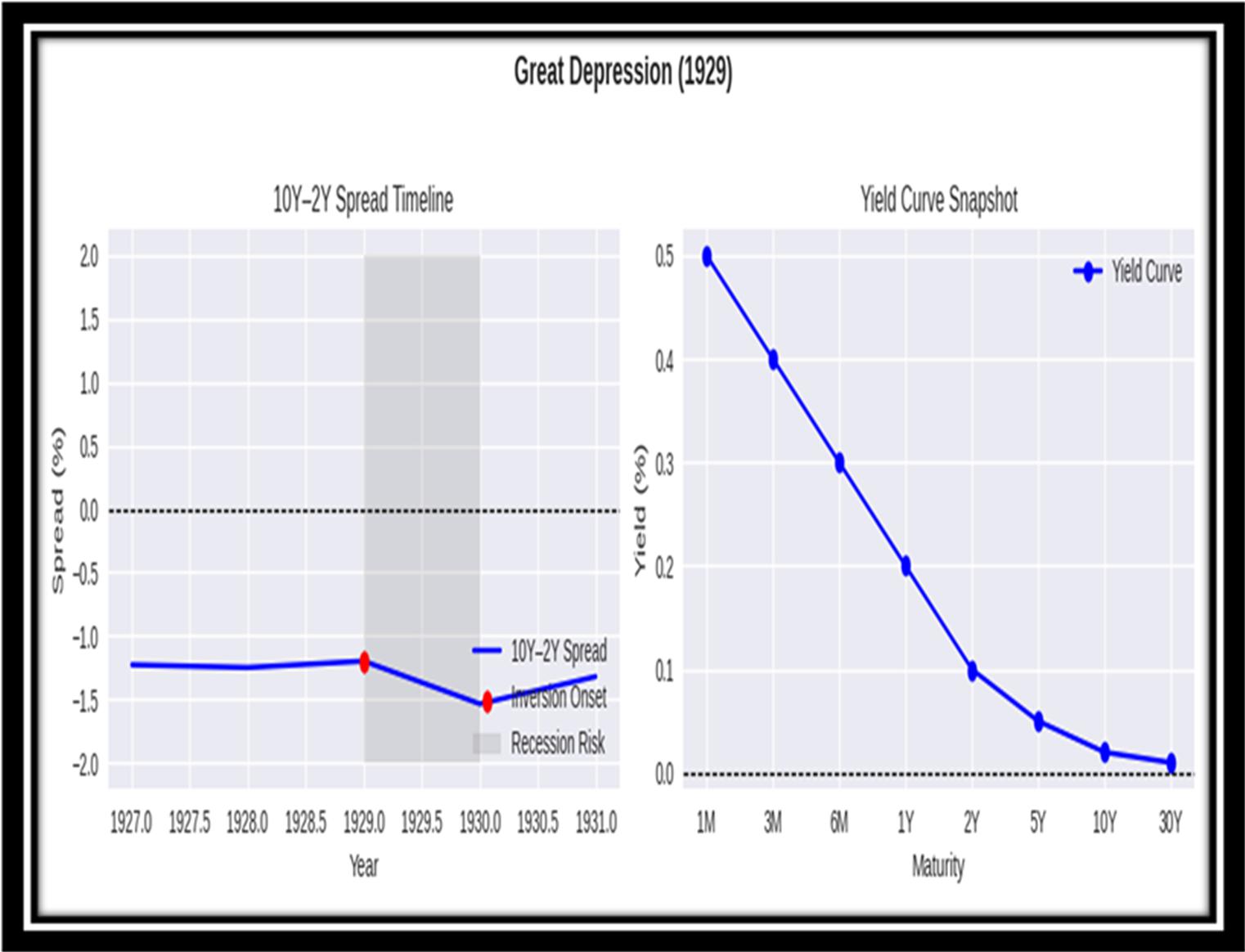
Figure 1a. Analog Circuit Model (L overload is understood—bigtime leverage).
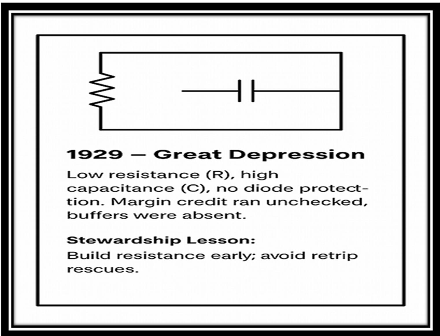
Figure2. 1973-75: Oil Embargo | Stagflation
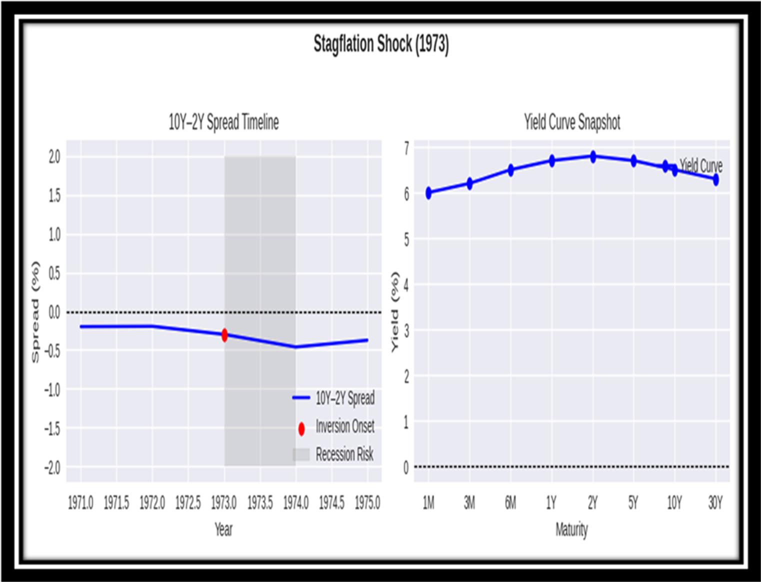
Figure 2a. Analog Circuit Model.
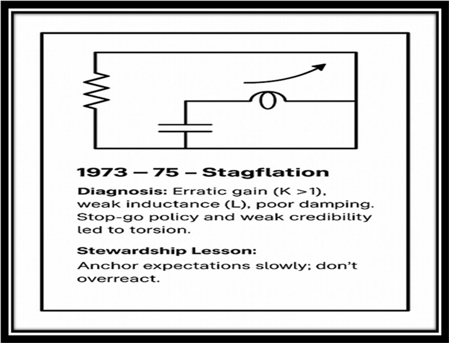
Figure 3. 1987: Flash Crash.
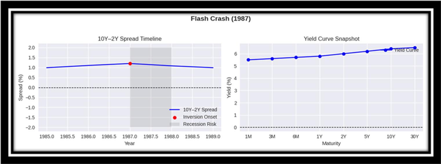
Figure 3a. Analog Circuit Model (no significant R or C, no L).
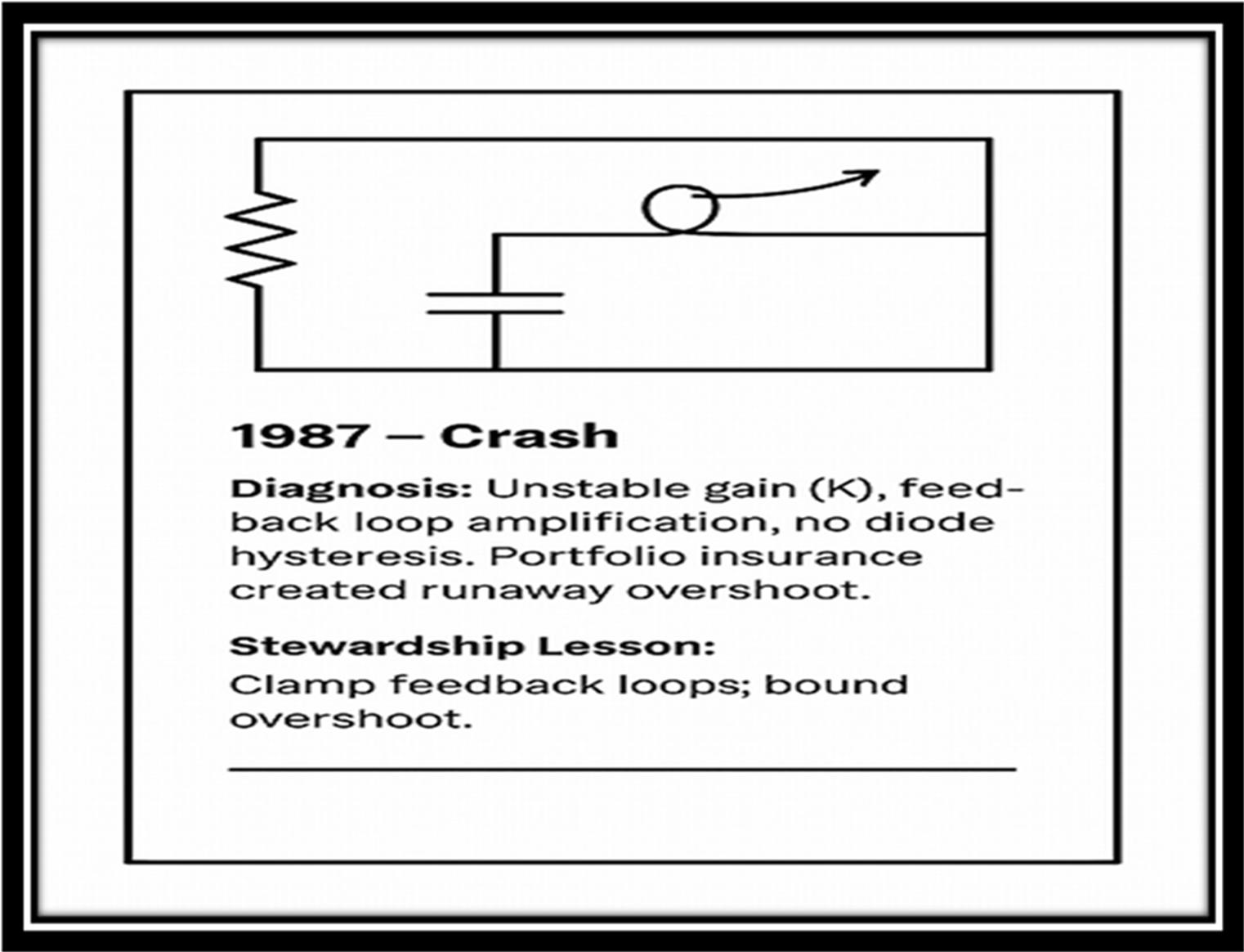
Figure 4. 1998: Dot-Com Setup
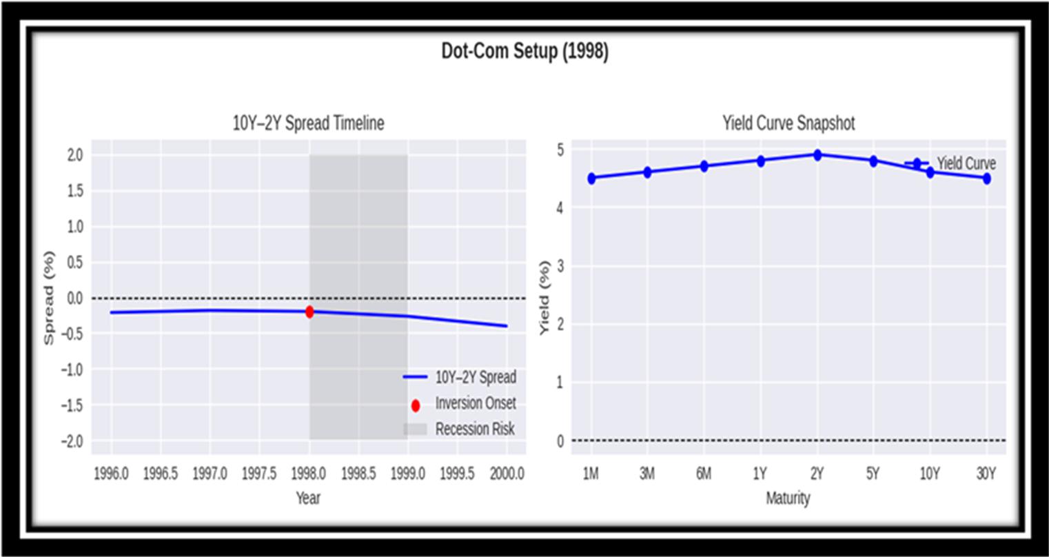
Figure 4a. Analog Circuit Model.
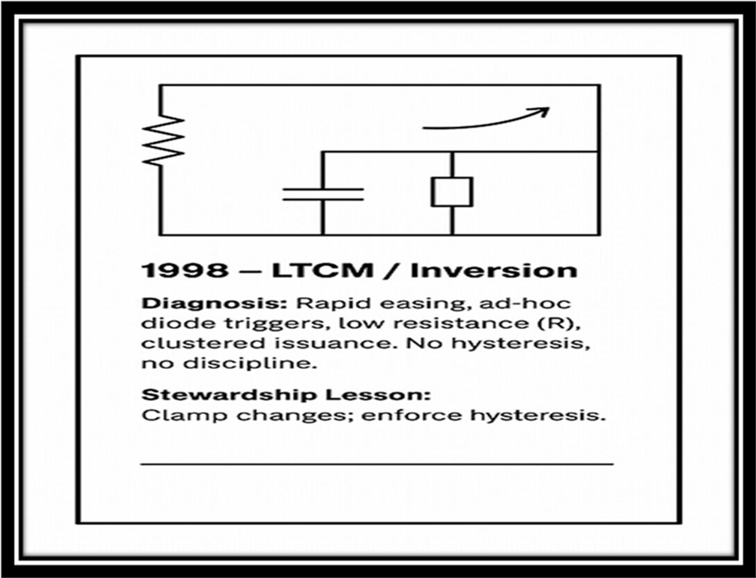
Figure 5. 2008: Banking | Financial Crisis.
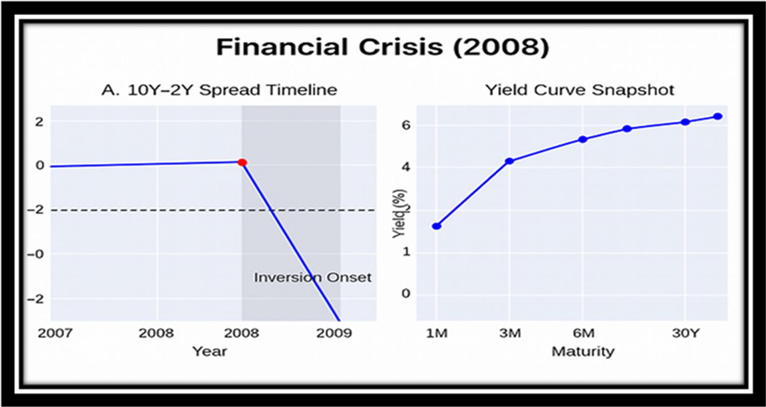
Figure 5a. Analog Circuit Model.
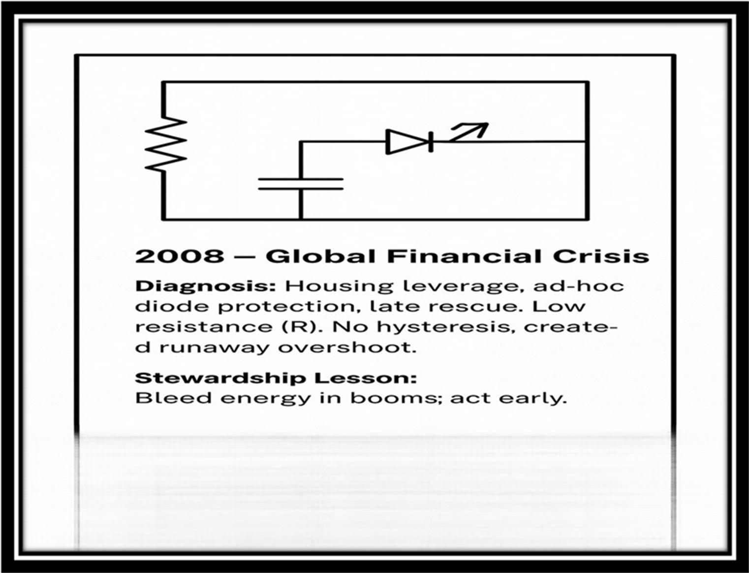
Figure 6. 2020: Pandemic Shock/Whiplash.
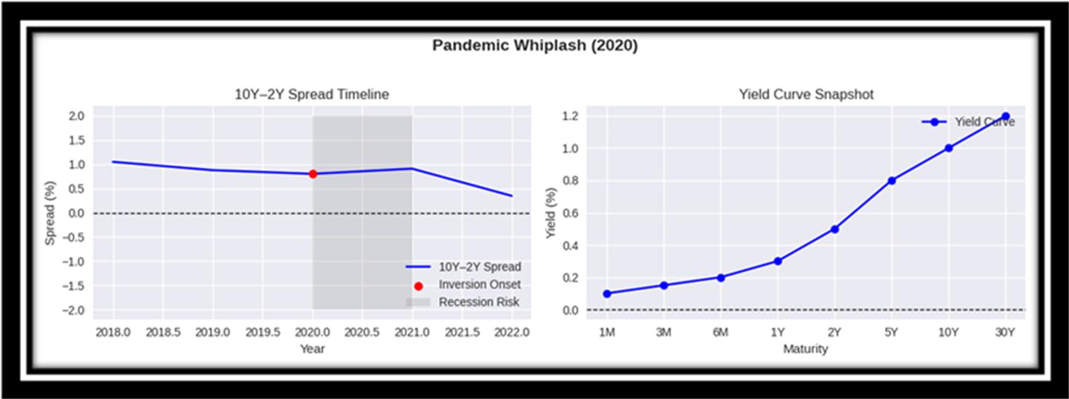
Figure 6a. Analog Circuit Model.

Figure 7. 2022ff: Deepest Inverstion/Spread to Date.
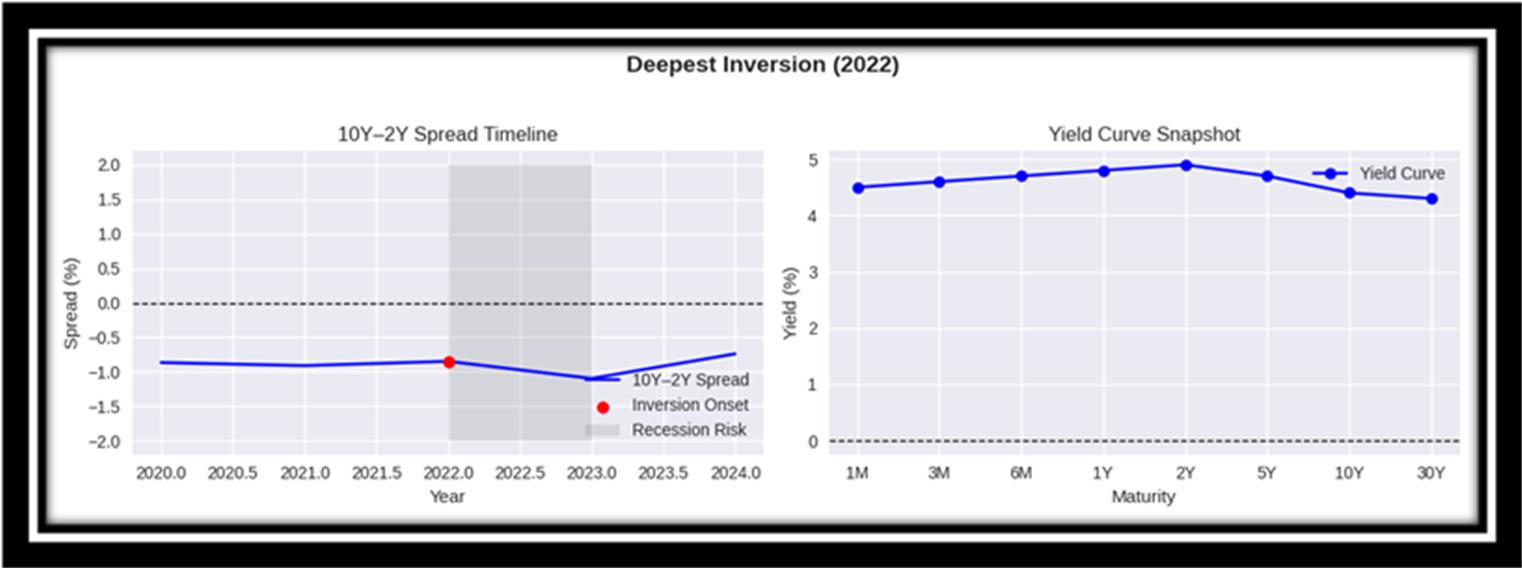
Figure 7a. Analog Circuit Model.
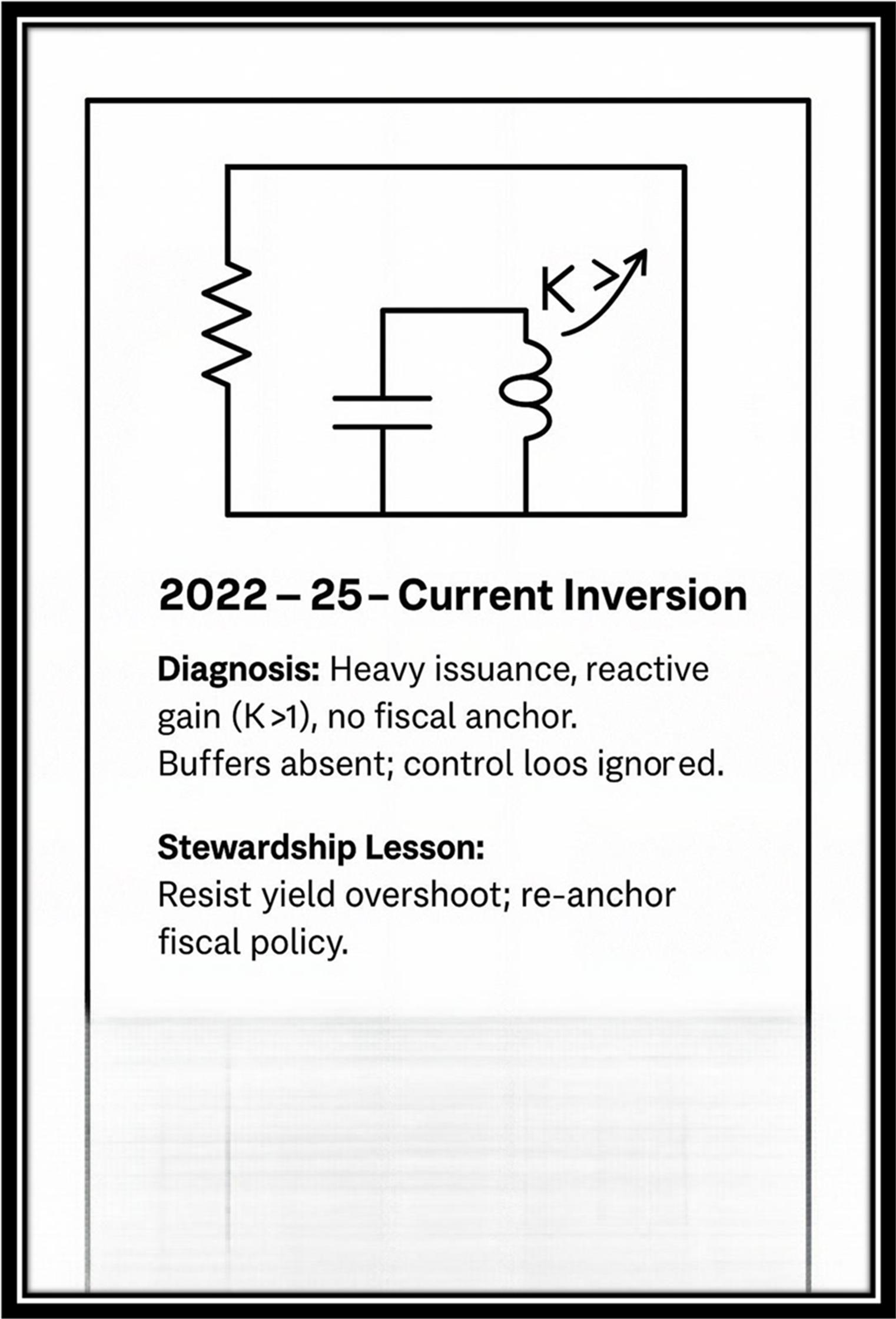
Figure 8. Shock Interval Decay Curve (explanation).
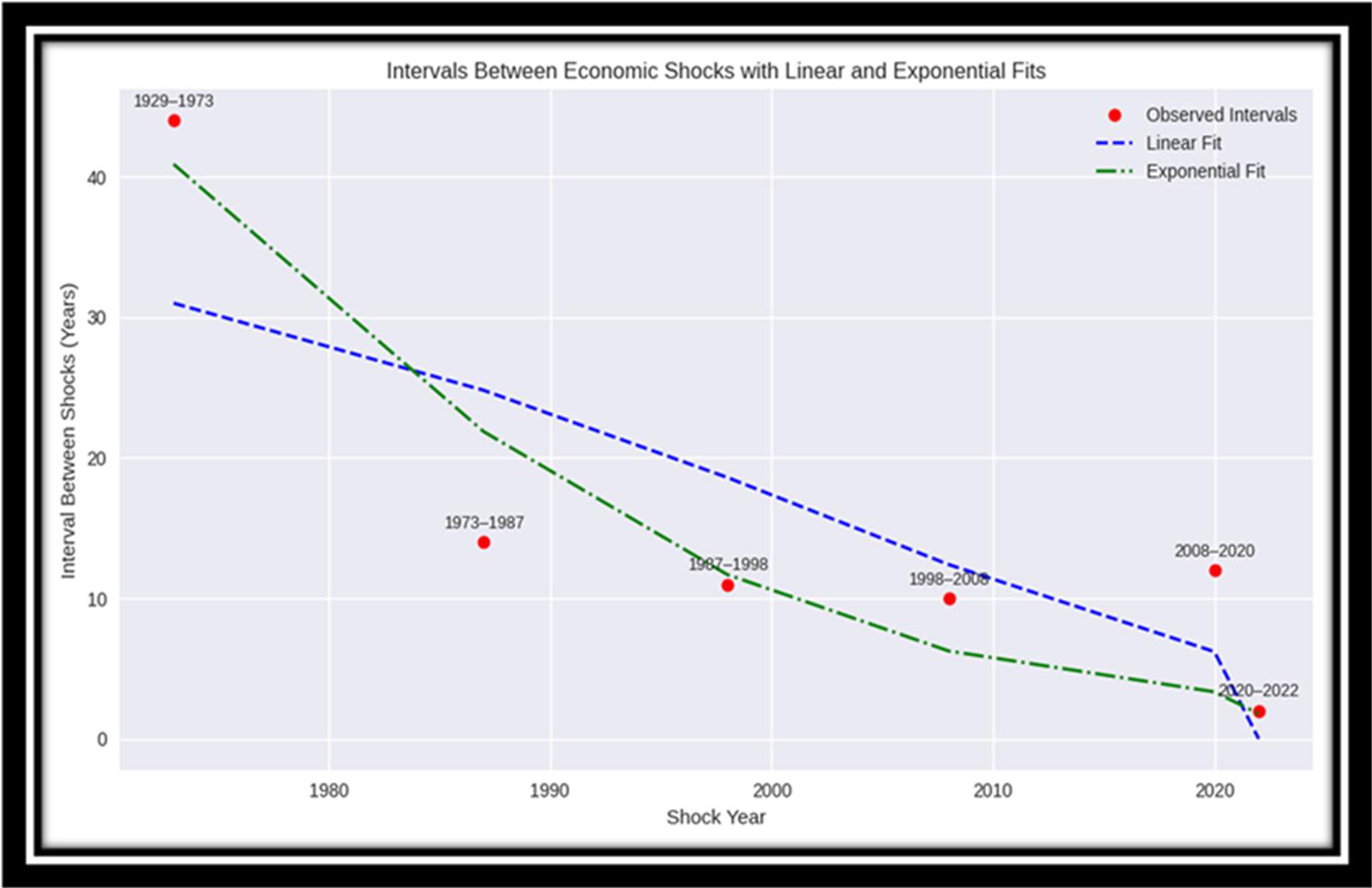
Concerning Figure 8 and shrinking intervals between major economic shocks (1929–2022ff). The plot shows crisis‑year intervals: {44, 14, 13, 8, 12, 2}, not yield curve inversion intervals: {4, 5, 11, 11, 6, 13, 3 for inversion years 1969, 1973, 1978, 1989, 2000, 2006, 2019, 2022 respectively}. Regression diagnostics confirm that crisis‑year intervals produce a much stronger fit (linear: blue/dashed, R² ≈0.65—explains about 65% of the variation; exponential green, R² ≈0.86—explains about 86% of the variation), than inversion‑based intervals (not shown; linear R² ≈0.02—explains about 2% of the variation, exponential R² ≈−0.05—effectively no explanatory power here; the negative value reflects that the exponential model performs worse than a flat mean). This makes clear that inversions are signals rather than precise crisis markers. For clarity and to present meaningful results we therefore report results based on crisis years, where the clustering pattern is most evident.
The crisis intervals show a clear shrinking pattern. The linear fit (blue, dashed, R² ≈0.65) suggests a steady decline but collapses unrealistically to zero. The exponential fit (green, R² ≈ 0.86) is a better fit and it captures an accelerating pattern where shocks cluster ever closer together[5]. But why use two data-fitting models (linear and exponential)? We are “testing” for ever‑shrinking time intervals between shocks. To see the pattern clearly, we need good resolution; if our “eyeball tool” is too coarse, we risk missing the real trend. For example, imagine driving past a row of trees at a constant speed. If the trees are spaced far apart, you see each one clearly, passing by at a steady rhythm. That’s what linear fitting does—it assumes changes happen at a constant pace. That’s how the blue/dashed curve was captured—a linear fit. But if the trees start getting closer together, you might miss some because your “eyeball tool” isn’t fine enough. That’s where exponential fitting comes in handy: now imagine you’re timing a race with a digital stopwatch. As the runners speed up, the stopwatch can still capture every split-second change. That’s exponential fitting—it’s designed to handle rapid, shrinking intervals, picking up details that a simple linear tool would miss. That’s how the green curve was captured—an exponential fit—and what was captured resembles exponential decay: it’s telling us that the data, i.e. the shock intervals, shorten rapidly but never vanish entirely—that’s classic exponential decay. The green curve is approaching zero asymptotically, implying ever tighter shock clustering going forward. As time ticks on, shocks will appear increasingly rapid‑fire unless something dramatic were to intervene to alter the trajectory. Sure, outliers will occur, but what the exponential fit makes abundantly clear is the accelerating pattern.
That said, there is a subtlety to note: the linear–exponential crossover—which occurs just before the 1973–1987 interval. At this point the exponential fit begins to drop below the linear fit, indicating that shocks are arriving faster than the linear model expects. The system is entering a decidedly feedback‑driven regime here: resolution matters much more, and accordingly the exponential model starts outperforming the linear one. Still, only the final interval (2020–2022) is tightly matched. Although several of the post‑crossover intervals (1973–2020) exhibit noticeable residuals, the exponential regression specification nonetheless reduces overall error variance and represents the accelerating trend more faithfully than the linear alternative. Statistically, the linear model implies a collapse to zero in finite time—an implausible projection—whereas the exponential model approaches zero only asymptotically, preserving interpretive plausibility and aligning more closely with the observed clustering of shocks.
Practically, the question is how can a crossover fifty years ago carry forward such economic sensitivity? The 1970s marked a structural break—a scar that never fully healed. Vietnam’s fiscal overhang (debt that hangs over government choices, limiting what policies can be made now and in the future), and the loss of perceived invincibility per the outcome of the war, followed by the oil embargo and heretofore unheard of loss of energy security, were global spectacles that revealed deep national vulnerabilities per an underlying fragility. Today’s tighter clustering of shocks reflects not just new crises, but the lingering fragility exposed back then, and that fragility is why the intervals’ exponential decay keeps holding post 1970s. Fragility has a way of feeding on itself: fragility reduces resilience, which which increases vulnerability and magnifies the impact of subsequent shocks, which further reduces resilience, and thus it loops since the 70s, holding the shock intervals’ exponential decay curve intact.
What condition is our nation’s condition in these days? The curves raise questions not only for economists but for all of us. And for those of us tethered to Jehovah God and His Word, they may even be understood as questions God is asking of our culture.
Table 1. Analog Circuits Guide.
| Shock Period
Jump to: 1929, 1973-75, 1987, 1998-2000, 2008, 2020, 2022, Fig. 8- shock interval decay curve. |
Circuit Logic | Diagnosis | Stewardship Lesson (with R, L, C adjustments) | ||||||||
| 1929 – Great Depression (Fig. 1, 1a) | We have here (1) Low to no R (damping), (2) igh C (stored up frothy energy: speculation, over the top valuations), (3) high L (lots of mojo), (4) no diode protection—energy flowed bigtime but in the wrong direction. 1929 maps most cleanly to a (second order) LC circuit and that baby can really ring—In economics, that’s the unstable feedback between speculative momentum (L) and stored froth (C) (see key). | “In 1929 the bus rolled downhill with no brakes R (ouch)—margin credit ran unchecked. The springs (L) carried momentum forward, and the tanks (C) were brimming with speculative froth and valuations—but with no damping to bleed it off (=dissipation), the whole pent-up reservoir discharged very violently. Given this mojo of high C and no R, the crash was literally baked in. | To keep the 1929 ride from wrecking, lay down some damping R right early so the wheels don’t spin out, and drain off the extra slosh in the tanks (C) so they don’t spill their contents all over the place like Mt. St. Helen’s, and set up a one‑way gate (diode) so the flow can’t run backward into another rescue. Consider Proverbs 10:5, 21:20. | ||||||||
| 1973–Stagflation Shock (Fig. 2, 2a) | We have here (1) Low R (monetary and fiscal policy slow to respond), (2) an unstable source (supply shock per the embargo), (3) weak L (this shock was predominantly driven by an exogenous event not speculative inertia), (4) a diode/s misfired (safeguards like energy reserves, diversification, or policy buffers didn’t kick in, the “diode” that should have blocked reverse flow or prevented back‑surges failed, allowing the shock to propagate through expectations, prices, and wages). This shock maps best to a first order RL circuit, hence we expect a long decay tail rather than oscillatory behavior—a dragged out affair was looming—poor damping R was to stretch the time constant tau=L/R (see key). | In 1973 the bus hit an oil slick. The springs (L) were weak—little inertia of their own—and the brakes (R) were too soft, so the jolt bled off slowly. With low damping, the shock stretched on and on, dragging mile after mile into an inflation spiral, all sparked by “…up from the ground came a bubblin’ crude…” | “To ride out the 1973 storm, you needed steady damping capacity (R) in the brakes, and keep the springs (L) weak so the bus doesn’t buck too hard when jolted, and patch up the one‑way gate (diode) so the flow (oil, liquidity) stays pointed forward instead of leaking backward into wages and prices. Consider Proverbs 11:1, 22:3. | ||||||||
| 1987–Flash Crash (Fig. 3, 3a) | We have here (1) Sudden voltage drop (input shock—program trading and a hedging strategy with a twist called portfolio insurance triggered rapid selloffs), (2) low to no L (an exogenous trigger amplified by feedback loops and automated trading), (3) no stabilizer diode to stop the bleeding once positive feedback took hold. Note: hysteresis + diode prevents such retrips. With no significant R or C, the circuit analog is best described as a low‑L, feedback‑driven system. The “ringing” here does not arise from second-order LC resonance but from recursive feedback amplification in the absence of stabilizers (see key). | In 1987 the cart outpaced the horse—program trading bolted ahead faster than human oversight could steer. The crash was amplified by positive feedback—runaway reflections in the feedback loops of portfolio insurance. There was little damping (R) on the wheels at the time—circuit breakers only came later—and no one‑way gate (diode) to stop flows from reversing violently. Futures and equities fed each other like two mirrors bouncing light back and forth, until the whole doggone thing spiraled itself into a ditch. | “To keep the 1987 bus from shakin’, rattlin’, and rollin’ itself into a ditch, you had to test for runaway reflections in the feedback loops. That meant strengthening the springs (L)—not to crank up oscillation but to give the bus enough stabilizing inertia so jolts get absorbed instead of bounced back. Then slap some serious damping R on the wheels so governance slows the spin (trading halts, circuit breakers), and for sure patch a one‑way gate (diode) so the flow can’t suddenly reverse and crash again. Consider Proverbs 11:14, 20:18. | ||||||||
| 1998–False Positive (Fig. 4, 4a) | We have here (1) A brief nerves-inversion (typical, very human, quick polarity flip—exuberance turned to doubt, ultimately to fear, and then panic—the short artist’s narrow window—valuations inverted and greed got ate up by fear), (2) low R (weak damping: governance and regulation didn’t slow speculative spin [high C]—IPO frenzy and loose capital weren’t slowed because of greed-driven oversight; R bleeds frenzy off, so speculators and even investors “hate” R because it reduces the payoff from rapid swings so on that layer the weak R was welcomed—gladly overlooked—on the system layer it was overlooked because, well, the (capitalist) system is tilted toward greed because the “growth” it produces “feels” like prosperity), (3) low to medium L (some inertia from investor optimism, but not enough to garner continuity, stability), (4) capacitor discharged like Vesuvius (the speculative reservoir got flushed—dot‑com valuations collapsed once confidence drained), (5) no hysteresis (provides memory and thresholds—it prevents a system from flipping back and forth at the slightest disturbance; with hysteresis, once you trip, you don’t immediately retrip—the system requires a bigger reversal to flip back; in this scenario investor sentiment flipped rapidly—exuberance to fear, greed to panic—with no stabilizing threshold). This here 1998 false positive is best modeled by an RLC circuit analog, but in a degenerate form—low R, low‑medium L, and a discharging C with no hysteresis. It’s a weakly damped RLC bubble‑burst system (see key). | In 1998 the bus looked steady, but only because the driver poured extra water through the pipes. The Fed’s liquidity flood masked cracks in the frame—the tanks (C) looked full, but the bearings were worn. It was a false positive: the flow seemed fine, but underneath, the ol’ bus was fragile, ready to rattle, screech, and seize up. | When the rig keeps on mistakin’ noise for a real signal, you gotta’ steady its springs (L) so they don’t bounce too wildly when jolted, and for sure tune them tanks (C) so they don’t slosh over when hit, and of course, add some damping (R) to hush the rattles. Then, then what? You screw on—glue and zip ties not allowed—a memory latch (hysteresis) so that once the thing trips, it won’t re‑trip until things really, really change. And last but not least, you set a one‑way gate (diode) so nothin’ sneaks back the wrong way (ouch). That way the rig listens to the true call and ignores them tantalizin’ false sirens. Consider Proverbs 14:18, 1John 4:1. | ||||||||
|
|
|
|
||||||||
| 2020–Pandemic Whiplash (Fig. 6, 6a) | We have here (1) speculative capacitance (excess liquidity—the Fed injected liquidity through massive asset purchases/QE, emergency lending facilities, and near‑zero interest rates, which “charged up” parallel tanks of speculative capacitance in markets), and (2) speculative positions per se (“overbuilt tanks” of leverage and risk), and (3) glaringly missing phase buffers (no staggered “valves”—release mechanisms like policy coordination or supply chain redundancy). When the pandemic shock hit, all the tanks dumped at once, and without strategically placed valves to slow or phase the release, the system flooded. (4) The markets had two big flips here (whiplash = health shock + liquidity shock), and they carried external momentum (inductance L—global supply chains, debt loads) that flat out resisted quick adjustment. Once jolted, the system carried forward a sort of rolling thunder shock inertia—momentum that kept volatility oscillating across coupled markets, amplified by delayed feedback between virus spread and policy response, even after the initial event. The circuit analog that best fits here is a multi‑capacitor, under‑damped RLC network with missing phase buffers and strong external inductive coupling. (see key). | When COVID slammed the brakes, the bus’s pipes froze up, and nothing was moving. So, the Fed opened the floodgates, pouring water through the system to keep the wheels turning. The ride got really messy and sloshy, but at least the bus didn’t seize up completely. | To steady this dripping rig, give ‘er bigger tanks (C) to hold the overflow, springs (L) to soak up the bumps, and a bit of damping (R) to keep it from rattling, and add a one‑way latch (diode) so nothing runs backward—and for goodness sake figure out where to place some release valves[7]; the whole contraption rides smoother that way when this sort of pain comes along again (God forbid). Consider Proverbs 6:6-8, 27:12. | ||||||||
| 2022ff–Deepest Inversion (Fig. 7, 7a) | We have here (1) prolonged reverse bias (from rapid Fed hikes) has held the “credit junction” in reverse, widening the depletion region and stalling forward flow. (2) With high inductance L from long‑term debt loads and global supply chains resisting quick adjustment, and (3) rising resistance from quantitative tightening and tighter credit standards, the system has become (4) phase‑lagged (delay between input change and system response, a function of inductance L/inertia and sluggish current flows and voltage adjustments [current sluggish to adjust across debt‑laden inductive branches, voltage levels sluggish to re‑stabilize across reserve‑laden capacitive branches], (5) Yield curve inversion flipped polarity across maturities, creating back‑pressure even on short branches, so attempts at “re‑conduction” sputter into stop‑start oscillations and occasional snapbacks rather than smooth recovery. The circuit that best fits here is a reverse‑biased, multi‑branch RLC network: a PN‑junction (policy stance) held in reverse bias, feeding a yield‑curve “ladder” of branches with mismatched sources, high inductance L (long‑horizon commitments), and rising resistance R (quantitative tightening). It’s under‑damped in transients (stop‑start oscillations, snapbacks) yet over‑damped for steady flow (stalled re‑conduction), producing phase‑lagged responses and back‑pressure across maturities (see key). | Fed hikes met with delayed market digestion; short end rose (voltage spike at the input), long end flattened (output flat refused to follow)—a kink-distortion with an attitude (on the long end) | To keep the bus from twisting itself out of shape, ease off the big springs (L) so it doesn’t buck too hard, steady the damping (R) so the wheels don’t wobble, and keep an eye on the tanks (C) so they don’t slosh over. That way the ride stays straight and doesn’t get distorted over the long haul.
A Quick Guide: Inductance (L): The big springs that carry momentum: If too high: Slow to turn, big bucks and overshoot. If too low: Twitchy; loses helpful momentum. Resistance (R): The damping that stabilizes motion. If too high: Feels stuck; forward flow stalls. If too low: Wobble, chatter, and oscillations. Capacitance (C): The tanks that store and smooth supply. If too high: Heavy slosh; slow rebalancing. If too low: Thin buffer; sharp jolts and shortages. A Quick Cue: Tune L (debt and supply chain inertia) for smooth turns, set R (credit friction damping) to kill wobble without stalling, size C (liquidity storage buffers) to cushion shocks without “boing”—bounce—and “slosh”—lingering drag. Consider 1Corinthians 4:2, 14:40). |
Note: The current deep yield inversion (2022ff) resembles a hybrid of post oil embargo 1978–79 (long duration, inflation‑driven Fed tightening, it was the longest yield inversion prior to the current one) and 1998–2000 (speculative excess, sentiment fragility). Unlike 1929 or 1987, today’s inversion is not a sudden crash but a drawn‑out imbalance. In a capitalist system, permissive oversight (low R) and absent hysteresis thresholds have allowed the inversion to persist unusually long, defying the usual recession timing. Pulling out will likely require both policy easing and structural reset—reflecting the combined fixes of 1978–79 and 2000. That would probably be something to watch/wait patiently for Christian friend. The precedent suggests that normalization[8] comes after policy easing and structural reset—not instantly, but in a cycle that rewards patience.
Works Cited and References
“A Letter of Invitation.”
Jesus, Amen.
< https://development.jesusamen.org/a-letter-of-invitation-2/ >
Analog Circuits: Hutters, C., & Mendel, M. B. (2024).
Economic Circuit Theory: Electrical Network Theory for Dynamical
Economic Systems.
IEEE Access,12, 172696-172713.
< https://doi.org/10.1109/ACCESS.2024.3465228 >
Analog Circuits: “Anological Models.”
Wikipedia.
< https://en.wikipedia.org/wiki/Analogical_models >
“God’s Exponential Framework.”
Jesus, Amen.
< https://development.jesusamen.org/gods-exponential-framework/ >
Microsoft.
Copilot AI Assistant.
November 2025.
1929: “The Crash of 1929.”
Bill of Rights Institute.
< https://billofrightsinstitute.org/essays/the-crash-of-1929 >
1929: “The Great Depression Analogy.”
National Bureau of Economic Research.
< https://www.nber.org/system/files/working_papers/w15584/w15584.pdf >
1973-75: “Understanding Stagflation: Lessons From the 1970s Economic Crisis.”
Investopedia.
< https://www.investopedia.com/articles/economics/08/1970 >
1973-75: “What is Stagflation and Why Does It Matter? When Inflation and Unemployment Rise Together.”
GovFacts.
1998-2000: “Dot-com Bubble Explained | Story of 1995-2000 Stock Market.”
Finbold.com
< https://finbold.com/guide/dot-com-bubble-crash/ >
1998-2000: “Understanding the Dotcom Bubble: Causes, Impact, and Lessons.”
Investopedia.
< https://www.investopedia.com/terms/d/dotcom-bubble.asp >
2008: “The Financial Crisis 2008 Explained in Simple Terms.”
Economyria.
< https://economyria.com/the-financial-crisis-2008-explained/ >
2008: “The 2008 Financial Crisis Explained.”
Investopedia.
< https://www.investopedia.com/articles/economics/09/financial-crisis-review.asp >
2020: “COVID-19 and the Economy: A Comprehensive Analysis.”
Michigan Journal of Economics.
< https://sites.lsa.umich.edu/mje/2024/11/25/covid-19-and-the-economy-a-comprehensive-analysis/ >
2020: “2020 Year in Review: The impact of COVID-19 in 12 charts.”
World Bank.
< https://blogs.worldbank.org/en/voices/2020-year-review-impact-covid-19-12-charts >
2022: “Is a Recession on the Horizon?”
OJM Group.
<https://www.ojmgroup.com/investment-commentary/yield-curve-inversions-explained-2022-update/ >
2022: “What Do Yield Curve Inversions Really Tell Us?”
Dimensional.
< https://www.dimensional.com/us-en/insights/what-do-yield-curve-inversions-really-tell-us >
Notes
[1] These are government programs and tax systems that kick in automatically to stabilize the economy during booms and busts, without requiring new laws or active intervention.
[2] Inductors embody “electrical inertia.” They’re like a heavy flywheel in electricity—they don’t let current change suddenly—that’s the big takeaway for the analogy. More technically, the coil builds a strong axial magnetic field that stores energy as current loops around (field lines spread outward, but the dominant, useful field is axial through the coil’s center). And here’s the high-plane beauty God made available to us: current and magnetic field are mutually dependent—a changing current requires a changing magnetic field and a changing magnetic field induces a response in current (Brother Faraday’s Law). Now, by Lenz’s Law (faith uncertain, undocumented), that induced emf always opposes the change, resisting impulses and enforcing stability (it has to oppose, always, to prevent runaway growth and preserve conservation of energy). Think of the magnetic field as the flywheel—the sluggard; when current tries to change suddenly, the magnetic field cannot follow instantly, because that would require an infinite induced emf across the coil—that’s not allowed in Jehovah God’s Economy.
[3] The phenomenon of uncontrolled oscillations, sometimes referred to as “ringing,” is trouble because it red flags a system that’s under‑damped. In both circuits and economies, unchecked oscillations can overshoot the rails—whether voltage limits or fiscal boundaries—and cause real damage or false triggers or spurious frequencies. Technically, oscillations involve at least two energy storage elements (e.g. RLC, where R does not store energy, it dissipates it) because oscillations are essentially a game of trading energy—it takes two to tango (second order); single energy storage element circuits (e.g. RC, RL) do not oscillate, they drag/lag (monotonic exponential).
[4] “Nominal” in this context means the rated or expected value under standard stress testing; nominal values are typically published with some tolerable +/- standard deviation—the outputs must stay within that tolerance under standard operating conditions otherwise the device or system is flawed and unsafe and quite unusable in the environs it claims to be able to operate in. That’s the overarching design goal always be it circuits or economies or just about anything—keep the outputs nominal.
[5] Feedback dynamics are at work; said mathematically, we are dealing with data (intervals) where the change in an interval—dx/dt—is proportional to the current state of the interval itself—kx—or dx/dt=
-kx for a decaying system (notice the feedback happening in x)—this is precisely exponential decay, where each shorter interval accelerates the next. The exponential fit thus reflects feedback compression, it’s not a statistical accident. (It is intuitively obvious that feedback is the heartbeat of God’s Economy—the Created Order—and the fingerprint it leaves behind is precisely e [“God’s Exponential Framework”]).
[6] In a less mathematical sense, shocks arrive closer together because structural fragility, global interdependence, and feedback loops have compressed the system’s response time. Once the scar of the 1970s revealed vulnerability, it set the stage for each subsequent crisis to propagate more rapidly, confirming the accelerating trajectory. Fragility, interdependence, and feedback have compressed response times so tightly that shocks risk arriving faster than resilience can rebuild. In statistical terms, the curve approaches zero asymptotically; in systemic terms, it hints at implosion. So, here is yet another curve that fits the title of our study: “The Curve and the Curse, Signals in a Fallen World.”
[7] Pareto analysis can be a useful starting point for the Fed to think about “release valves,” since it highlights the few critical nodes that drive most systemic risk. In circuit terms, it’s like identifying the handful of capacitors or inductors that store most of the system’s energy and then placing resistors or phase buffers at those points to prevent catastrophic discharge. By focusing on the 20% of vulnerabilities that create 80% of instability—such as leverage in shadow banking, liquidity mismatches, or concentrated speculative positions—the Fed could design staggered interventions that relieve pressure where it matters most. That said, Pareto analysis alone isn’t sufficient. Financial markets are dynamic, and small nodes can cascade if tightly coupled. To build a robust release‑valve strategy, Pareto prioritization should be complemented by stress testing (simulating shocks across the whole circuit) and network analysis (mapping contagion pathways between markets). Together, these approaches provide both focus and resilience: Pareto shows where to place the valves, while stress tests and network maps ensure the system won’t surprise policymakers with hidden weak points.
[8] When short‑term interest rates fall back below long‑term rates, the yield curve “normalizes.” That steepening signals confidence that inflation is cooling and growth can continue without immediate recession. In plain terms: the financial system stops running upside‑down, and borrowing costs look healthier again. But yield curve steepening is a tricky thing—it takes experience to assess it aright, it’s not a standalone green light.